Object-based time series image analysis

Object-Based Image Analysis (OBIA) is an approach to remote sensing image analysis that partitions an image into closed segments which are then classified and analyzed. For high-resolution images (1 meter or smaller) the aim of OBIA is to create objects that represent meaningful features in the real world, like buildings, roads, fields, forests, and water bodies. In case of medium resolution images (such as Sentinel-2 or Landsat) the segments represent groups of the image with similar spectral responses which in general do not correspond directly to individual objects in the ground. These groups of pixels are called super-pixels. In both situations, the aim of OBIA is to obtain a spatial partition of the image which can then be assigned to a single class. When applicable, OBIA reduces processing time and produces labeled maps with greater spatial consistency.

The general sequence of the processes involved in OBIA in sits is:

Segmentation: The first step is to group together pixels that are similar based a distance metric that considers the values of all bands in all time instances. We build a multitemporal attribute space where each time/band combination is taken as an independent dimension. Thus, distance metrics for segmentation in a data cube with 10 bands and 24 time steps use a 240-dimension space.
Probability Estimation: After the image has been partitioned into distinct objects, the next step is to classify each segment. For satellite image time series, a subset of time series inside each segment is classified.
Labeling: Once the set of probabilities have been obtained for each time series inside a segment, they can be used for labeling. This is done by considering the median value of the probabilities for the time series inside the segment that have been classified. For each class, we take the median of the probability values. Then, median values for the classes are normalised, and the most likely value is assigned as the class for the segment.

Image segmentation in sits

The first step of the OBIA procedure in sits is to select a data cube to be segmented and function that performs the segmentation. For this purpose, sits provides a generic sits_segment() function, which allows users to select different segmentation algorithms. The sits_segment() function has the following parameters:

cube: a regular data cube.
seg_fn: function to apply the segmentation
roi: spatial region of interest in the cube
start_date: starting date for the space-time segmentation
end_date: final date for the space-time segmentation
memsize: memory available for processing
multicores: number of cores available for processing
output_dir: output directory for the resulting cube
version: version of the result
progress: show progress bar?

In sits version 1.4.2, there is only one segmentation function available (sits_slic) which implements the extended version of the Simple Linear Iterative Clustering (SLIC) which is described below. In future versions of sits, we expect to include additional functions that support spatio-temporal segmentation.

Simple linear iterative clustering algorithm

After building the multidimensional space, we use the Simple Linear Iterative Clustering (SLIC) algorithm [92] that clusters pixels to efficiently generate compact, nearly uniform superpixels. This algorithm has been adapted by Nowosad and Stepinski [93] to work with multispectral images. SLIC uses spectral similarity and proximity in the image space to segment the image into superpixels. Superpixels are clusters of pixels with similar spectral responses that are close together, which correspond to coherent object parts in the image. Here’s a high-level view of the extended SLIC algorithm:

The algorithm starts by dividing the image into a grid, where each cell of the grid will become a superpixel.
For each cell, the pixel in the center becomes the initial “cluster center” for that superpixel.
For each pixel, the algorithm calculates a distance to each of the nearby cluster centers. This distance includes both a spatial component (how far the pixel is from the center of the superpixel in terms of x and y coordinates) and a spectral component (how different the pixel’s spectral values are from the average values of the superpixel). The spectral distance is calculated using all the temporal instances of the bands.
Each pixel is assigned to the closest cluster. After all pixels have been assigned to clusters, the algorithm recalculates the cluster centers by averaging the spatial coordinates and spectral values of all pixels within each cluster.
Steps 3-4 are repeated for a set number of iterations, or until the cluster assignments stop changing.

The outcome of the SLIC algorithm is a set of superpixels which try to capture the to boundaries of objects within the image. The SLIC implementation in sits 1.4.1 uses the supercells R package [93]. The parameters for the sits_slic() function are:

dist_fn: metric used to calculate the distance between values. By default, the “euclidean” metric is used. Alternatives include “jsd” (Jensen-Shannon distance), and “dtw” (dynamic time warping) or one of 46 distance and similarity measures implemented in the R package philentropy [94].
avg_fn: function to calculate a value of each superpixel. There are two internal functions implemented in C++ - “mean” and “median”. It is also possible to provide a user-defined R function that returns one value based on an R vector.
step: distance, measured in the number of cells, between initial superpixels’ centers.
compactness: A value that controls superpixels’ density. Larger values cause clusters to be more compact.
minarea: minimal size of the output superpixels (measured in number of cells).

Example of SLIC-based segmentation and classification

To show an example of SLIC-based segmentation, we first build a data cube, using images available in the sitsdata package.

# directory where files are located
data_dir <- system.file("extdata/Rondonia-20LMR", package = "sitsdata")
# Builds a cube based on existing files
cube_20LMR <- sits_cube(
  source = "AWS",
  collection = "SENTINEL-2-L2A",
  data_dir = data_dir,
  progress = FALSE
)
plot(cube_20LMR, red = "B11", green = "B8A", blue = "B02", date = "2022-07-16")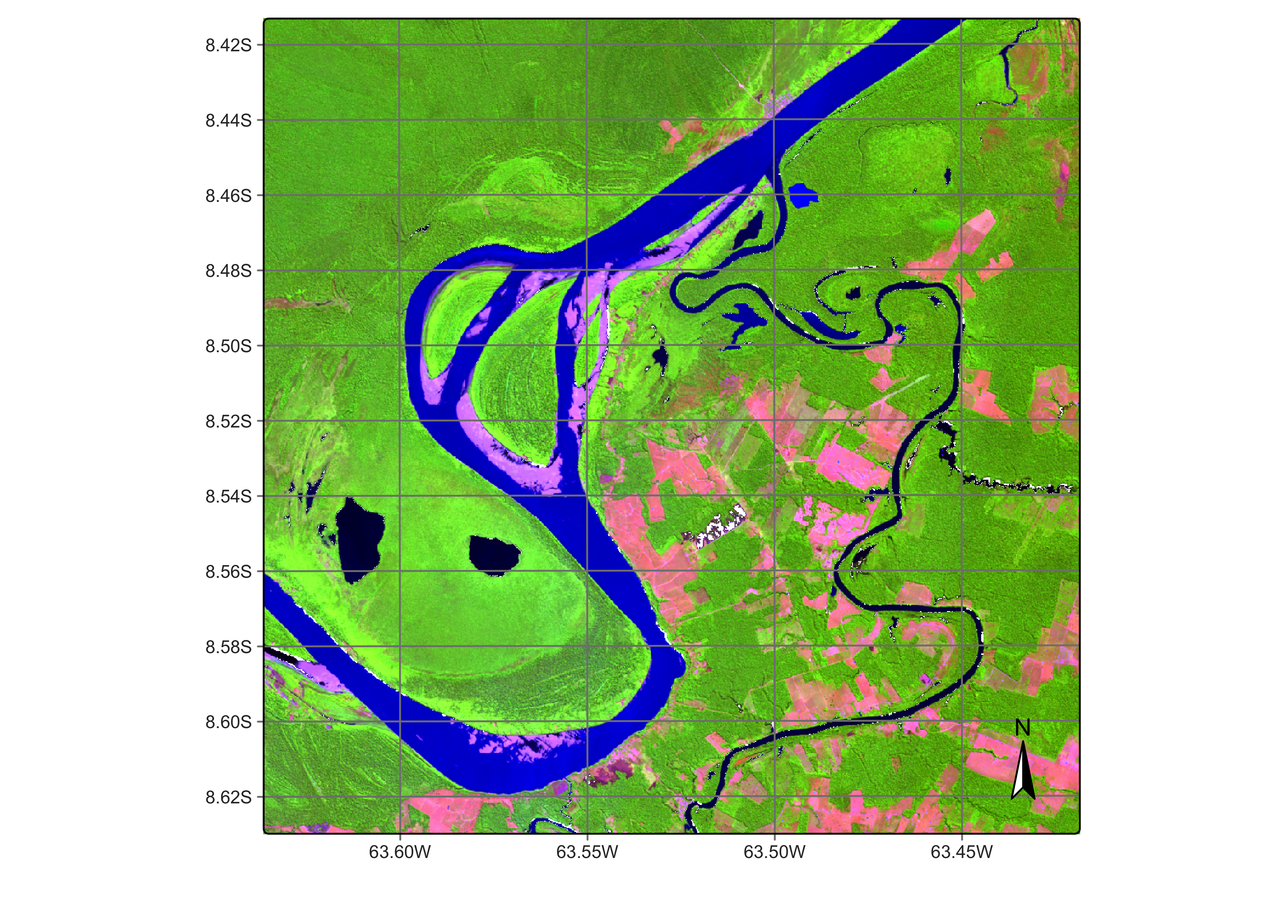

Figure 94: Sentinel-2 image in an area of Rondonia in Brazil

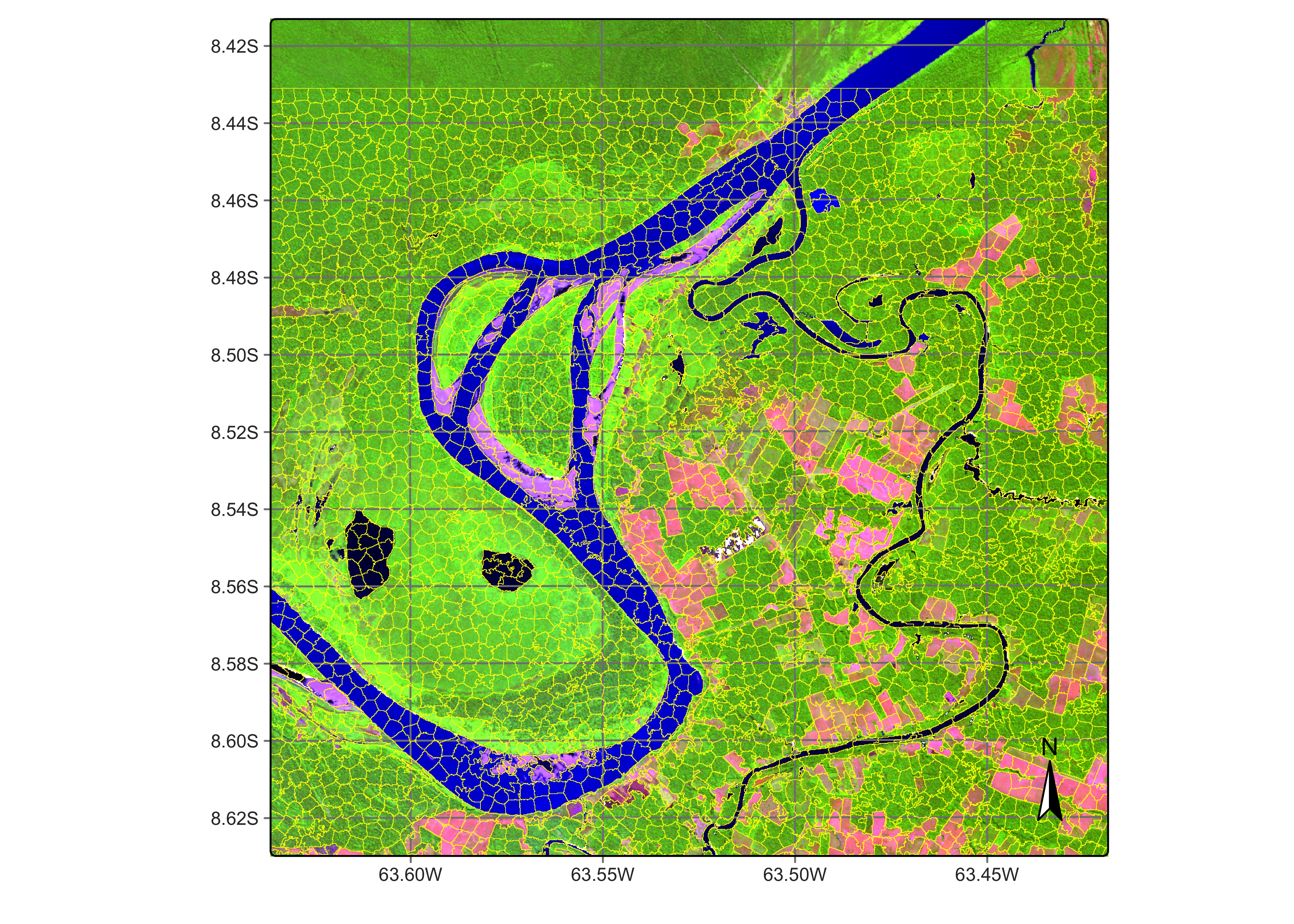
The following example produces a segmented image. For the SLIC algorithm, we take the initial separation between cluster centres (step) to be 20 pixels, the compactness to be 1, and the minimum area for each superpixel (min_area) to be 20 pixels.

# segment a cube using SLIC
# Files are available in a local directory
segments_20LMR <- sits_segment(
  cube = cube_20LMR,
  output_dir = "./tempdir/chp14",
  seg_fn = sits_slic(
    step = 20,
    compactness = 1,
    dist_fun = "euclidean",
    iter = 20,
    minarea = 20
  )
)
plot(segments_20LMR,
  red = "B11", green = "B8A", blue = "B02",
  date = "2022-07-16"
)

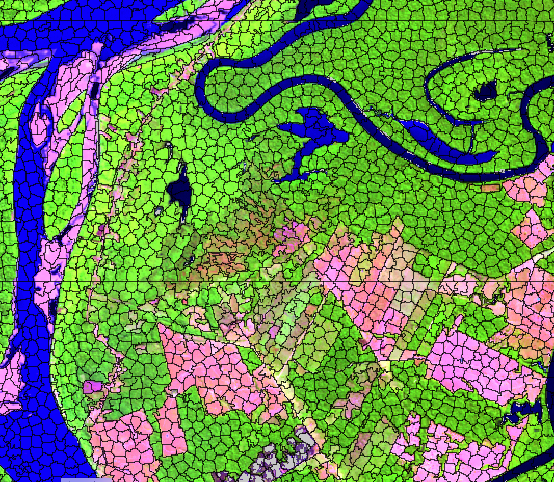
It is useful to visualize the segments in a leaflet together with the RGB image using sits_view().

sits_view(segments_20LMR,
  red = "B11", green = "B8A", blue = "B02",
  dates = "2022-07-16"
)

After obtaining the segments, the next step is to classify them. This is done by first training a classification model. In this case study, we will use an SVM model.

svm_model <- sits_train(samples_deforestation, sits_svm())

The segment classification procedure applies the model to a number of user-defined samples inside each segment. Each of these samples is then assigned a set of probability values, one for each class. We then obtain the median value of the probabilities for each class and normalize them. The output of the procedure is a vector data cube containing a set of classified segments. The parameters for the sits_classify()

segments_20LMR_probs_svm <- sits_classify(
  data = segments_20LMR,
  ml_model = svm_model,
  output_dir = "./tempdir/chp14",
  n_sam_pol = 40,
  gpu_memory = 16,
  memsize = 24,
  multicores = 6,
  version = "svm-segments"
)

segments_20LMR_class_svm <- sits_label_classification(
  segments_20LMR_probs_svm,
  output_dir = "./tempdir/chp14",
  memsize = 24,
  multicores = 6,
  version = "svm-segments"
)

To view the classified segments together with the original image, use plot() or sits_view(), as in the following example.

sits_view(
  segments_20LMR_class_svm,
  red = "B11",
  green = "B8A",
  blue = "B02",
  dates = "2022-07-16",
)

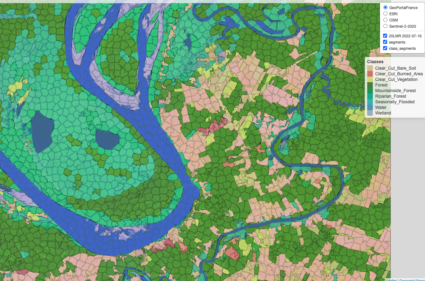
We conclude that OBIA analysis applied to image time series is a worthy and efficient technique for land classification, combining the desirable sharp object boundary properties required by land use and cover maps with the analytical power of image time series.

Ensemble prediction from multiple models

Technical annex