Machine learning for data cubes

Machine learning classification

Machine learning classification is a type of supervised learning in which an algorithm is trained to predict which class an input data point belongs to. The goal of machine learning models is to approximate a function \(y = f(x)\) that maps an input \(x\) to a class \(y\). A model defines a mapping \(y = f(x;\theta)\) and learns the value of the parameters \(\theta\) that result in the best function approximation [45]. The difference between the different algorithms is their approach to building the mapping that classifies the input data.
In sits, machine learning is used to classify individual time series using the time-first approach. The package includes two kinds of methods for time series classification:

1. Machine learning algorithms that do not explicitly consider the temporal structure of the time series. They treat time series as a vector in a high-dimensional feature space, taking each time series instance as independent from the others. They include random forest (sits_rfor()), support vector machine (sits_svm()), extreme gradient boosting (sits_xgboost()), and multilayer perceptron (sits_mlp()).

2. Deep learning methods where temporal relations between observed values in a time series are taken into account. These models are specifically designed for time series. The temporal order of values in a time series is relevant for the classification model. From this class of models, sits supports 1D convolution neural networks (sits_tempcnn()), residual 1D networks (sits_resnet()), and temporal attention-based encoders (sits_tae() and sits_lighttae()).

Based on experience with sits, random forest, extreme gradient boosting, and temporal deep learning models outperform SVM and multilayer perceptron models. The reason is that some dates provide more information than others in the temporal behavior of land classes. For instance, when monitoring deforestation, dates corresponding to forest removal actions are more informative than earlier or later dates. Similarly, a few dates may capture a large portion of the variation in crop mapping. Therefore, classification methods that consider the temporal order of samples are more likely to capture the seasonal behavior of image time series. Random forest and extreme gradient boosting methods that use individual measures as nodes in decision trees can also capture specific events such as deforestation.

The following examples show how to train machine learning methods and apply them to classify a single time series. We use the set samples_matogrosso_mod13q1, containing time series samples from the Brazilian Mato Grosso state obtained from the MODIS MOD13Q1 product. It has 1,892 samples and nine classes (Cerrado, Forest, Pasture, Soy_Corn, Soy_Cotton, Soy_Fallow, Soy_Millet). Each time series covers 12 months (23 data points) with six bands (NDVI, EVI, BLUE, RED, NIR, MIR). The samples are arranged along an agricultural year, starting in September and ending in August. The dataset was used in the paper “Big Earth observation time series analysis for monitoring Brazilian agriculture” [46], being available in the R package sitsdata.

Common interface to machine learning and deep learning models

The sits_train() function provides a standard interface to all machine learning models. This function takes two mandatory parameters: the training data (samples) and the ML algorithm (ml_method). After the model is estimated, it can classify individual time series or data cubes with sits_classify(). In what follows, we show how to apply each method to classify a single time series. Then, in Chapter Image classification in data cubes, we discuss how to classify data cubes.

Since sits is aimed at remote sensing users who are not machine learning experts, it provides a set of default values for all classification models. These settings have been chosen based on testing by the authors. Nevertheless, users can control all parameters for each model. Novice users can rely on the default values, while experienced ones can fine-tune model parameters to meet their needs. Model tuning is discussed at the end of this Chapter.

When a set of time series organized as tibble is taken as input to the classifier, the result is the same tibble with one additional column (“predicted”), which contains the information on the labels assigned for each interval. The results can be shown in text format using the function sits_show_prediction() or graphically using plot().

Random forest

Random forest is a machine learning algorithm that uses an ensemble learning method for classification tasks. The algorithm consists of multiple decision trees, each trained on a different subset of the training data and with a different subset of features. To make a prediction, each decision tree in the forest independently classifies the input data. The final prediction is made based on the majority vote of all the decision trees. The randomness in the algorithm comes from the random subsets of data and features used to train each decision tree, which helps to reduce overfitting and improve the accuracy of the model. This classifier measures the importance of each feature in the classification task, which can be helpful in feature selection and data visualization. Pelletier et al. discuss the robustness of random forest method for satellite image time series classification [47].

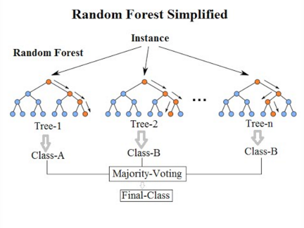
Figure 45: Random forest algorithm (Source: Venkata Jagannath in Wikipedia - licenced as CC-BY-SA 4.0).

sits provides sits_rfor(), which uses the R randomForest package [48]; its main parameter is num_trees, which is the number of trees to grow with a default value of 100. The model can be visualized using plot().

# Train the Mato Grosso samples with random forest model
rfor_model <- sits_train(
  samples = samples_matogrosso_mod13q1,
  ml_method = sits_rfor(num_trees = 100)
)
# Plot the most important variables of the model
plot(rfor_model)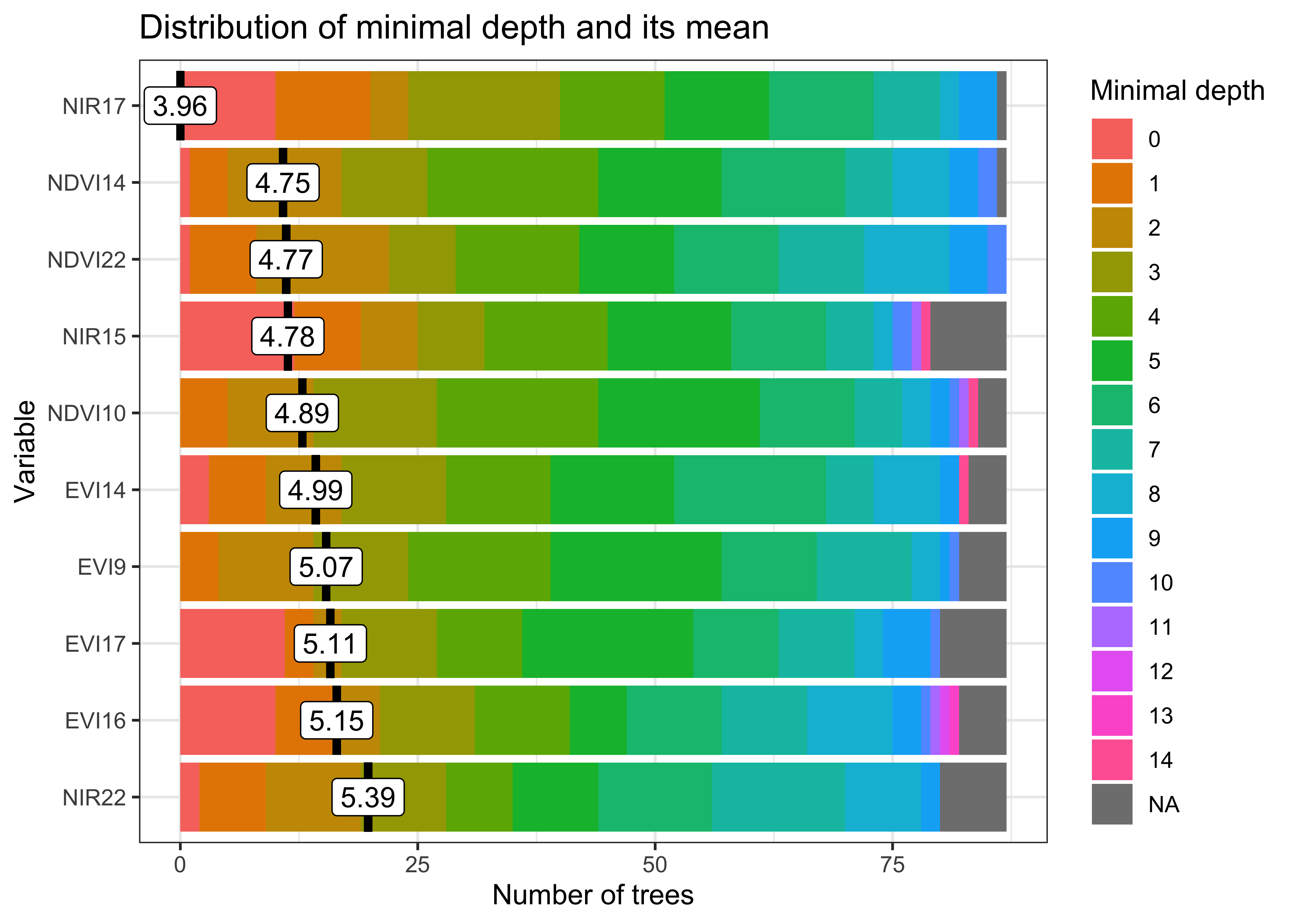

Figure 46: Most important variables in random forest model (Source: Authors).

The most important explanatory variables are the NIR (near infrared) band on date 17 (2007-05-25) and the MIR (middle infrared) band on date 22 (2007-08-13). The NIR value at the end of May captures the growth of the second crop for double cropping classes. Values of the MIR band at the end of the period (late July to late August) capture bare soil signatures to distinguish between agricultural and natural classes. This corresponds to summertime when the ground is drier after harvesting crops.

# Classify using random forest model and plot the result
point_class <- sits_classify(
  data = point_mt_mod13q1,
  ml_model = rfor_model
)
plot(point_class, bands = c("NDVI", "EVI"))

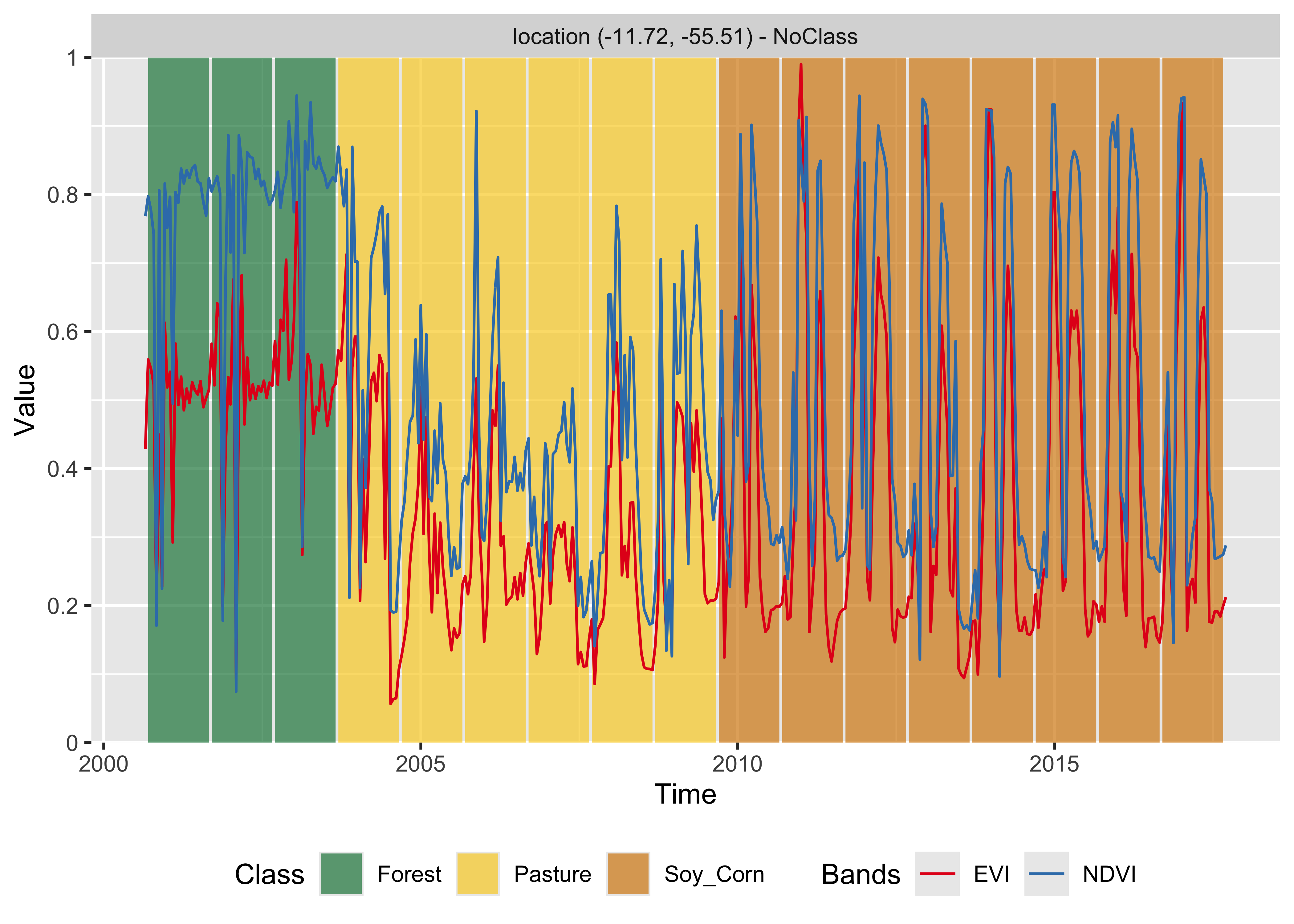
Figure 47: Classification of time series using random forest (Source: Authors).

The result shows that the area started as a forest in 2000, was deforested from 2004 to 2005, used as pasture from 2006 to 2007, and for double-cropping agriculture from 2009 onwards. This behavior is consistent with expert evaluation of land change process in this region of Amazonia.

Random forest is robust to outliers and can deal with irrelevant inputs [31]. The method tends to overemphasize some variables because its performance tends to stabilize after part of the trees is grown [31]. In cases where abrupt change occurs, such as deforestation mapping, random forest (if properly trained) will emphasize the temporal instances and bands that capture such quick change.

Support vector machine

The support vector machine (SVM) classifier is a generalization of a linear classifier that finds an optimal separation hyperplane that minimizes misclassification [49]. Since a set of samples with \(n\) features defines an n-dimensional feature space, hyperplanes are linear \({(n-1)}\)-dimensional boundaries that define linear partitions in that space. If the classes are linearly separable on the feature space, there will be an optimal solution defined by the maximal margin hyperplane, which is the separating hyperplane that is farthest from the training observations [50]. The maximal margin is computed as the smallest distance from the observations to the hyperplane. The solution for the hyperplane coefficients depends only on the samples that define the maximum margin criteria, the so-called support vectors.

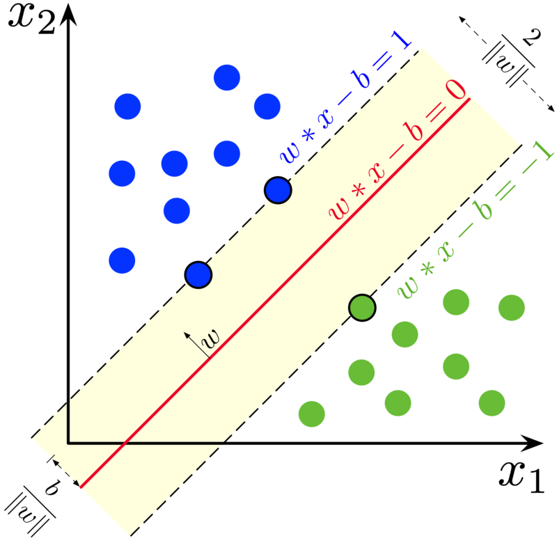
Figure 48: Maximum-margin hyperplane and margins for an SVM trained with samples from two classes. Samples on the margin are called the support vectors. (Source: Larhmam in Wikipedia - licensed as CC-BY-SA-4.0).

For data that is not linearly separable, SVM includes kernel functions that map the original feature space into a higher dimensional space, providing nonlinear boundaries to the original feature space. Despite having a linear boundary on the enlarged feature space, the new classification model generally translates its hyperplane to a nonlinear boundary in the original attribute space. Kernels are an efficient computational strategy to produce nonlinear boundaries in the input attribute space; thus, they improve training-class separation. SVM is one of the most widely used algorithms in machine learning applications and has been applied to classify remote sensing data [51].

In sits, SVM is implemented as a wrapper of e1071 R package that uses the LIBSVM implementation [52]. The sits package adopts the one-against-one method for multiclass classification. For a \(q\) class problem, this method creates \({q(q-1)/2}\) SVM binary models, one for each class pair combination, testing any unknown input vectors throughout all those models. A voting scheme computes the overall result.

The example below shows how to apply SVM to classify time series using default values. The main parameters are kernel, which controls whether to use a nonlinear transformation (default is radial), cost, which measures the punishment for wrongly-classified samples (default is 10), and cross, which sets the value of the k-fold cross validation (default is 10).

# Train an SVM model
svm_model <- sits_train(
  samples = samples_matogrosso_mod13q1,
  ml_method = sits_svm()
)
# Classify using the SVM model and plot the result
point_class <- sits_classify(
  data = point_mt_mod13q1,
  ml_model = svm_model
)
# Plot the result
plot(point_class, bands = c("NDVI", "EVI"))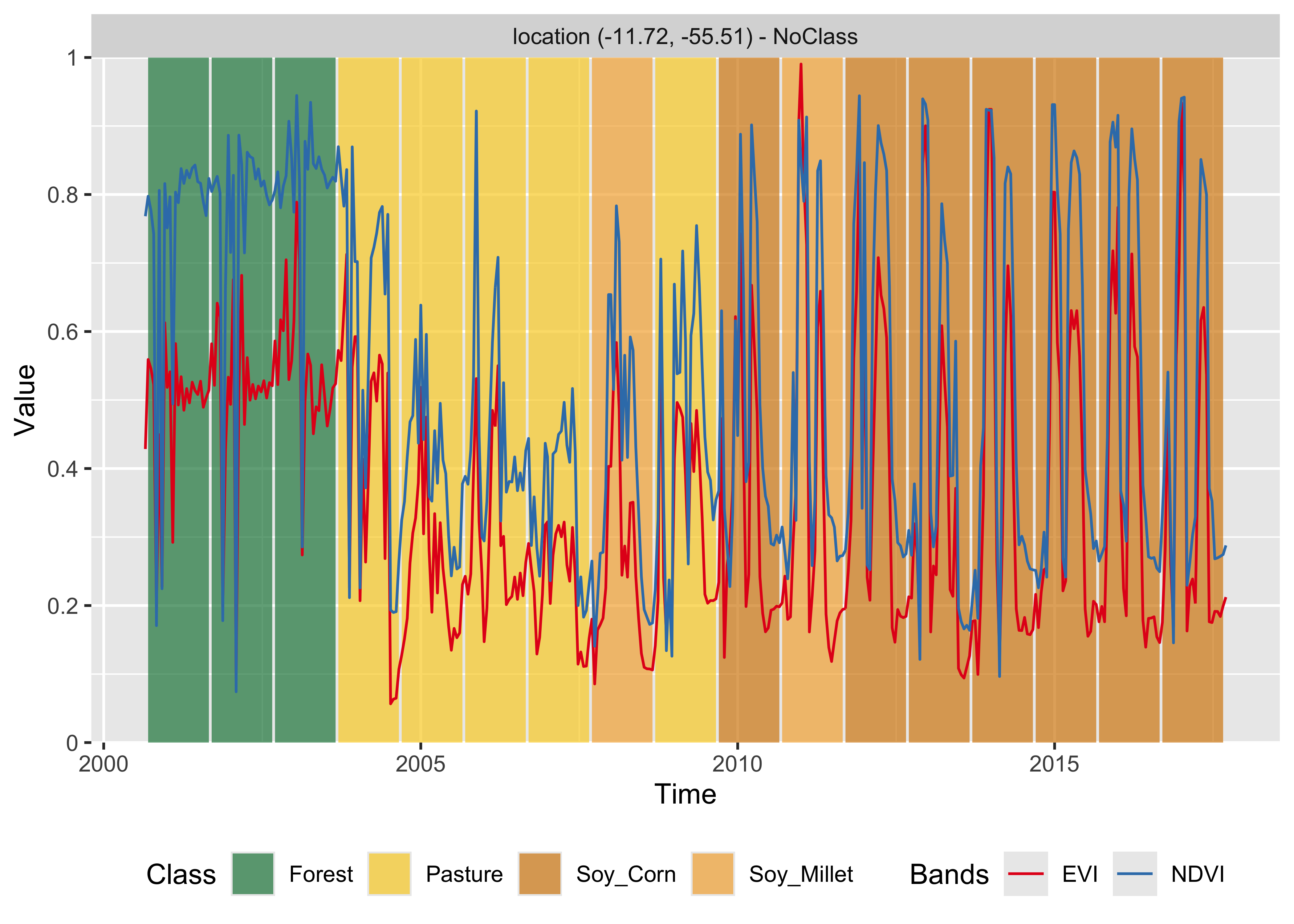

Figure 49: Classification of time series using SVM (Source: Authors).

The SVM classifier is less stable and less robust to outliers than the random forest method. In this example, it tends to misclassify some of the data. In 2008, it is likely that the correct land class was still Pasture rather than Soy_Millet as produced by the algorithm, while the Soy_Cotton class in 2012 is also inconsistent with the previous and latter classification of Soy_Corn.

Extreme gradient boosting

XGBoost (eXtreme Gradient Boosting) [53] is an implementation of gradient boosted decision trees designed for speed and performance. It is an ensemble learning method, meaning it combines the predictions from multiple models to produce a final prediction. Xgboost builds trees one at a time, where each new tree helps to correct errors made by previously trained tree. Each tree builds a new model to correct the errors made by previous models. Using gradient descent, the algorithm iteratively adjusts the predictions of each tree by focusing on instances where previous trees made errors. Models are added sequentially until no further improvements can be made.

Although random forest and boosting use trees for classification, there are significant differences. While random forest builds multiple decision trees in parallel and merges them together for a more accurate and stable prediction, xgboost builds trees one at a time, where each new tree helps to correct errors made by previously trained tree. XGBoost is often preferred for its speed and performance, particularly on large datasets, and is well-suited for problems where precision is paramount. Random Forest, on the other hand, is simpler to implement, more interpretable, and can be more robust to overfitting, making it a good choice for general-purpose applications.

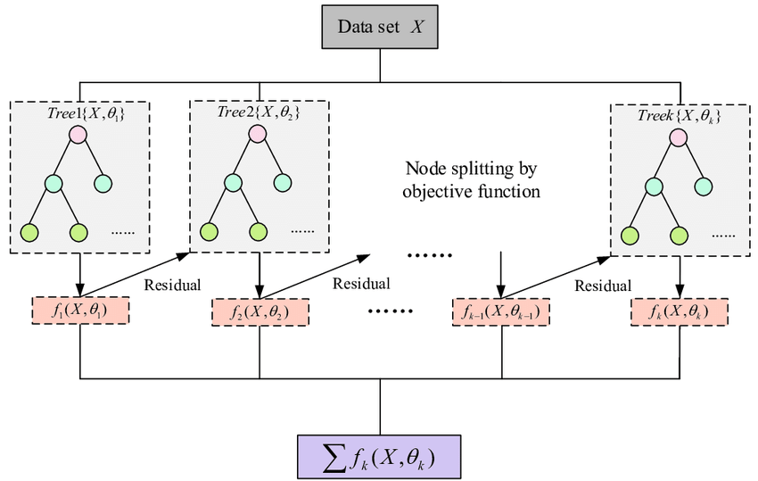
Figure 50: Flow chart of XGBoost algorithm (Source: Guo et al.,Applied Sciences, 2020. - licenced as CC-BY-SA 4.0).

The boosting method starts from a weak predictor and then improves performance sequentially by fitting a better model at each iteration. It fits a simple classifier to the training data and uses the residuals of the fit to build a predictor. Typically, the base classifier is a regression tree. Although random forest and boosting use trees for classification, there are significant differences. The performance of random forest generally increases with the number of trees until it becomes stable. Boosting trees apply finer divisions over previous results to improve performance [31]. Some recent papers show that it outperforms random forest for remote sensing image classification [54]. However, this result is not generalizable since the quality of the training dataset controls actual performance.

In sits, the XGBoost method is implemented by the sits_xbgoost() function, based on XGBoost R package, and has five hyperparameters that require tuning. The sits_xbgoost() function takes the user choices as input to a cross-validation to determine suitable values for the predictor.

The learning rate eta varies from 0.0 to 1.0 and should be kept small (default is 0.3) to avoid overfitting. The minimum loss value gamma specifies the minimum reduction required to make a split. Its default is 0; increasing it makes the algorithm more conservative. The max_depth value controls the maximum depth of the trees. Increasing this value will make the model more complex and likely to overfit (default is 6). The subsample parameter controls the percentage of samples supplied to a tree. Its default is 1 (maximum). Setting it to lower values means that xgboost randomly collects only part of the data instances to grow trees, thus preventing overfitting. The nrounds parameter controls the maximum number of boosting interactions; its default is 100, which has proven to be enough in most cases. To follow the convergence of the algorithm, users can turn the verbose parameter on. In general, the results using the extreme gradient boosting algorithm are similar to the random forest method.

# Train using  XGBoost
xgb_model <- sits_train(
  samples = samples_matogrosso_mod13q1,
  ml_method = sits_xgboost(verbose = 0)
)
# Classify using SVM model and plot the result
point_class_xgb <- sits_classify(
  data = point_mt_mod13q1,
  ml_model = xgb_model
)
plot(point_class_xgb, bands = c("NDVI", "EVI"))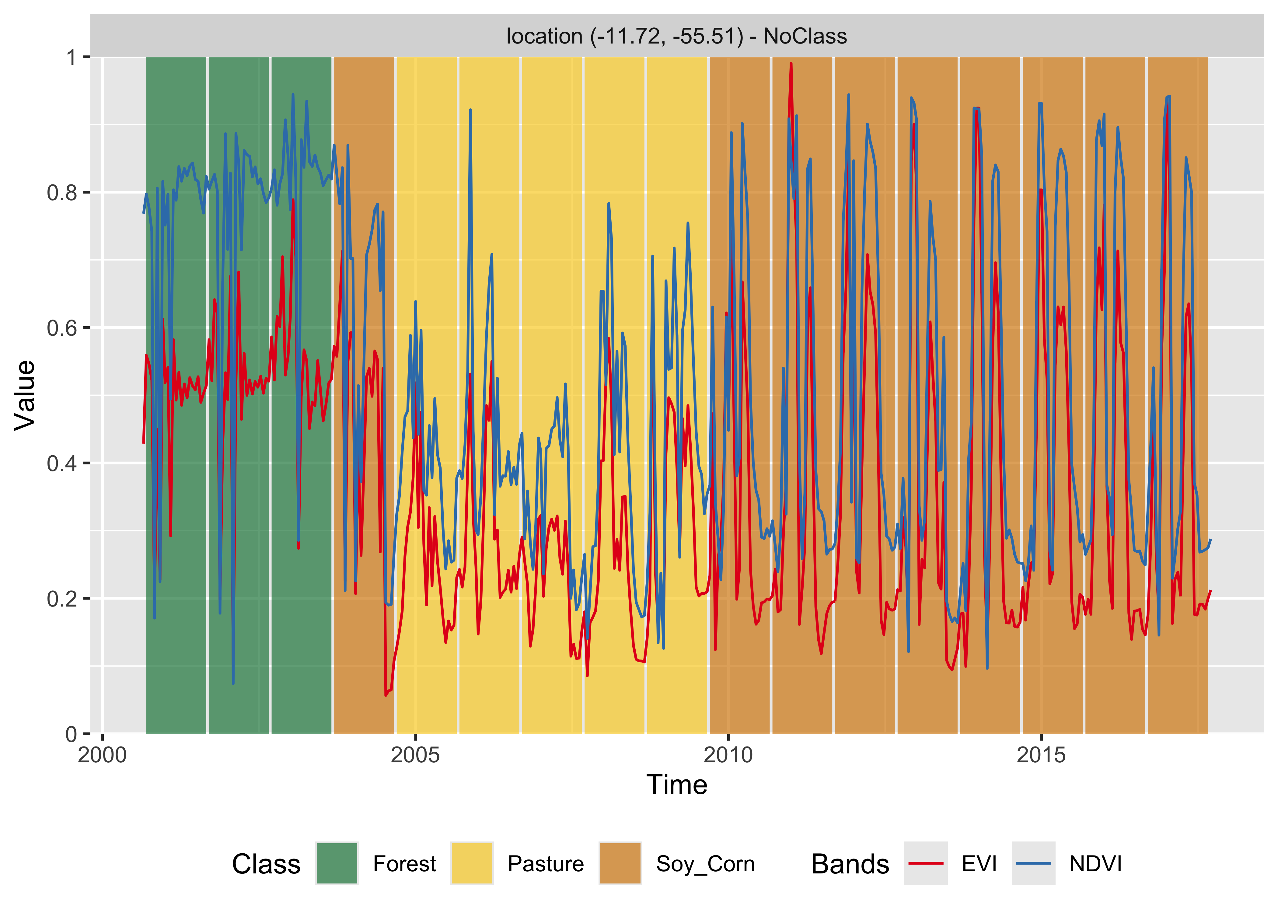

Figure 51: Classification of time series using XGBoost (Source: Authors).

Deep learning using multilayer perceptron

To support deep learning methods, sits uses the torch R package, which takes the Facebook torch C++ library as a back-end. Machine learning algorithms that use the R torch package are similar to those developed using PyTorch. The simplest deep learning method is multilayer perceptron (MLP), which are feedforward artificial neural networks. An MLP consists of three kinds of nodes: an input layer, a set of hidden layers, and an output layer. The input layer has the same dimension as the number of features in the dataset. The hidden layers attempt to approximate the best classification function. The output layer decides which class should be assigned to the input.

In sits, MLP models can be built using sits_mlp(). Since there is no established model for generic classification of satellite image time series, designing MLP models requires parameter customization. The most important decisions are the number of layers in the model and the number of neurons per layer. These values are set by the layers parameter, which is a list of integer values. The size of the list is the number of layers, and each element indicates the number of nodes per layer.

The choice of the number of layers depends on the inherent separability of the dataset to be classified. For datasets where the classes have different signatures, a shallow model (with three layers) may provide appropriate responses. More complex situations require models of deeper hierarchy. Models with many hidden layers may take a long time to train and may not converge. We suggest to start with three layers and test different options for the number of neurons per layer before increasing the number of layers. In our experience, using three to five layers is a reasonable compromise if the training data has a good quality. Further increase in the number of layers will not improve the model.

MLP models also need to include the activation function. The activation function of a node defines the output of that node given an input or set of inputs. Following standard practices [45], we use the relu activation function.

The optimization method (optimizer) represents the gradient descent algorithm to be used. These methods aim to maximize an objective function by updating the parameters in the opposite direction of the gradient of the objective function [55]. Based on experience with image time series, we recommend to start using the default method provided by sits, which is optimizer_adamw, from package torchopt. Please refer to the torchopt package for additional information.

Another relevant parameter is the list of dropout rates (dropout). Dropout is a technique for randomly dropping units from the neural network during training [56]. By randomly discarding some neurons, dropout reduces overfitting. Since a cascade of neural nets aims to improve learning as more data is acquired, discarding some neurons may seem like a waste of resources. In practice, dropout prevents an early convergence to a local minimum [45]. We suggest users experiment with different dropout rates, starting from small values (10-30%) and increasing as required.

The following example shows how to use sits_mlp(). The default parameters have been chosen based on a modified version of [57], which proposes using multilayer perceptron as a baseline for time series classification. These parameters are: (a) Three layers with 512 neurons each, specified by the parameter layers; (b) Using the “relu” activation function; (c) dropout rates of 40%, 30%, and 20% for the layers; (d) the “optimizer_adamw” as optimizer (default value); (e) a number of training steps (epochs) of 100; (f) a batch_size of 64, which indicates how many time series are used for input at a given step; and (g) a validation percentage of 20%, which means 20% of the samples will be randomly set aside for validation.

To simplify the output, the verbose option has been turned off. After the model has been generated, we plot its training history.

# Train using an MLP model
# This is an example of how to set parameters
# First-time users should test default options first
mlp_model <- sits_train(
  samples = samples_matogrosso_mod13q1,
  ml_method = sits_mlp(
    layers           = c(512, 512, 512),
    dropout_rates    = c(0.40, 0.30, 0.20),
    epochs           = 100,
    batch_size       = 64,
    verbose          = FALSE,
    validation_split = 0.2
  )
)
# Show training evolution
plot(mlp_model)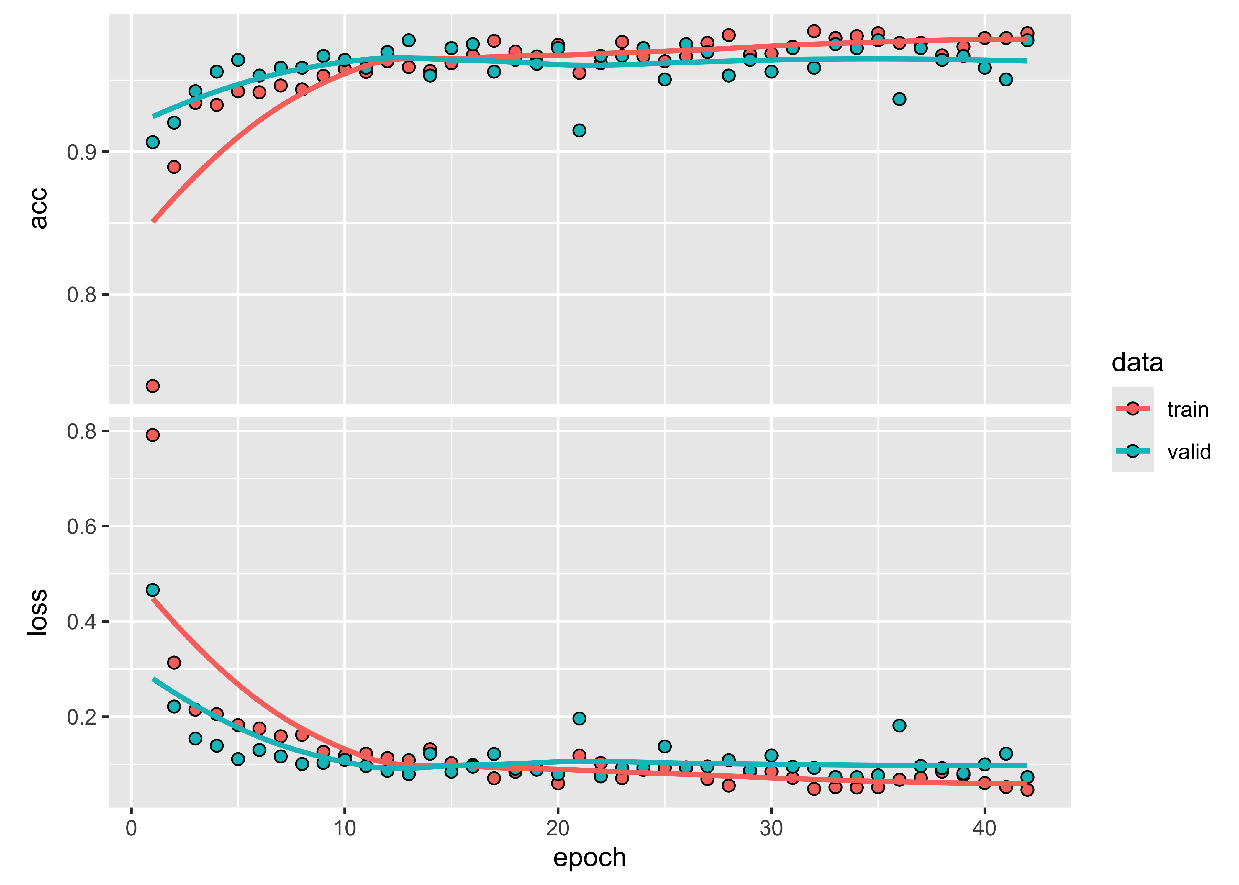

Figure 52: Evolution of training accuracy of MLP model (Source: Authors).

Then, we classify a 16-year time series using the multilayer perceptron model.

# Classify using MLP model and plot the result
point_mt_mod13q1 |>
  sits_classify(mlp_model) |>
  plot(bands = c("NDVI", "EVI"))

Figure 53: Classification of time series using MLP (Source: Authors).

In theory, multilayer perceptron model can capture more subtle changes than random forest and XGBoost In this specific case, the result is similar to theirs. Although the model mixes the Soy_Corn and Soy_Millet classes, the distinction between their temporal signatures is quite subtle. Also, in this case, this suggests the need to improve the number of samples. In this example, the MLP model shows an increase in sensitivity compared to previous models. We recommend to compare different configurations since the MLP model is sensitive to changes in its parameters.

Temporal Convolutional Neural Network (TempCNN)

Convolutional neural networks (CNN) are deep learning methods that apply convolution filters (sliding windows) to the input data sequentially. The Temporal Convolutional Neural Network (TempCNN) is a neural network architecture specifically designed to process sequential data such as time series. In the case of time series, a 1D CNN applies a moving temporal window to the time series to produce another time series as the result of the convolution.

TempCNN applies one-dimensional convolutions on the input sequence to capture temporal dependencies, allowing the network to learn long-term dependencies in the input sequence. Each layer of the model captures temporal dependencies at a different scale. Due to its multi-scale approach, TempCNN can capture complex temporal patterns in the data and produce accurate predictions.

The TempCNN architecture for satellite image time series classification is proposed by Pelletier et al. [58]. It has three 1D convolutional layers and a final softmax layer for classification (see Figure 54). The authors combine different methods to avoid overfitting and reduce the vanishing gradient effect, including dropout, regularization, and batch normalization. In the TempCNN reference paper [58], the authors favourably compare their model with the Recurrent Neural Network proposed by Russwurm and Körner [59]. Figure 54 shows the architecture of the TempCNN model.

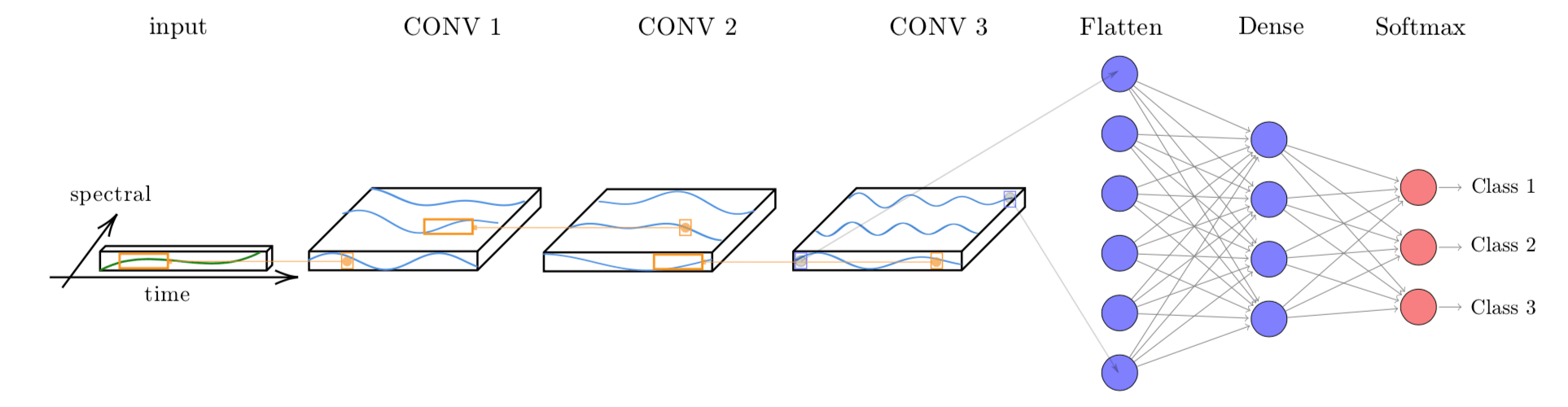
Figure 54: Structure of tempCNN architecture (Source: Pelletier et al. (2019). Reproduction under fair use doctrine).

The function sits_tempcnn() implements the model. The parameter cnn_layers controls the number of 1D-CNN layers and the size of the filters applied at each layer; the default values are three CNNs with 128 units. The parameter cnn_kernels indicates the size of the convolution kernels; the default is kernels of size 7. Activation for all 1D-CNN layers uses the “relu” function. The dropout rates for each 1D-CNN layer are controlled individually by the parameter cnn_dropout_rates. The validation_split controls the size of the test set relative to the full dataset. We recommend setting aside at least 20% of the samples for validation.

library(torchopt)
# Train using tempCNN
tempcnn_model <- sits_train(
  samples_matogrosso_mod13q1,
  sits_tempcnn(
    optimizer            = torchopt::optim_adamw,
    cnn_layers           = c(128, 128, 128),
    cnn_kernels          = c(7, 7, 7),
    cnn_dropout_rates    = c(0.2, 0.2, 0.2),
    epochs               = 100,
    batch_size           = 64,
    validation_split     = 0.2,
    verbose              = FALSE
  )
)
# Show training evolution
plot(tempcnn_model)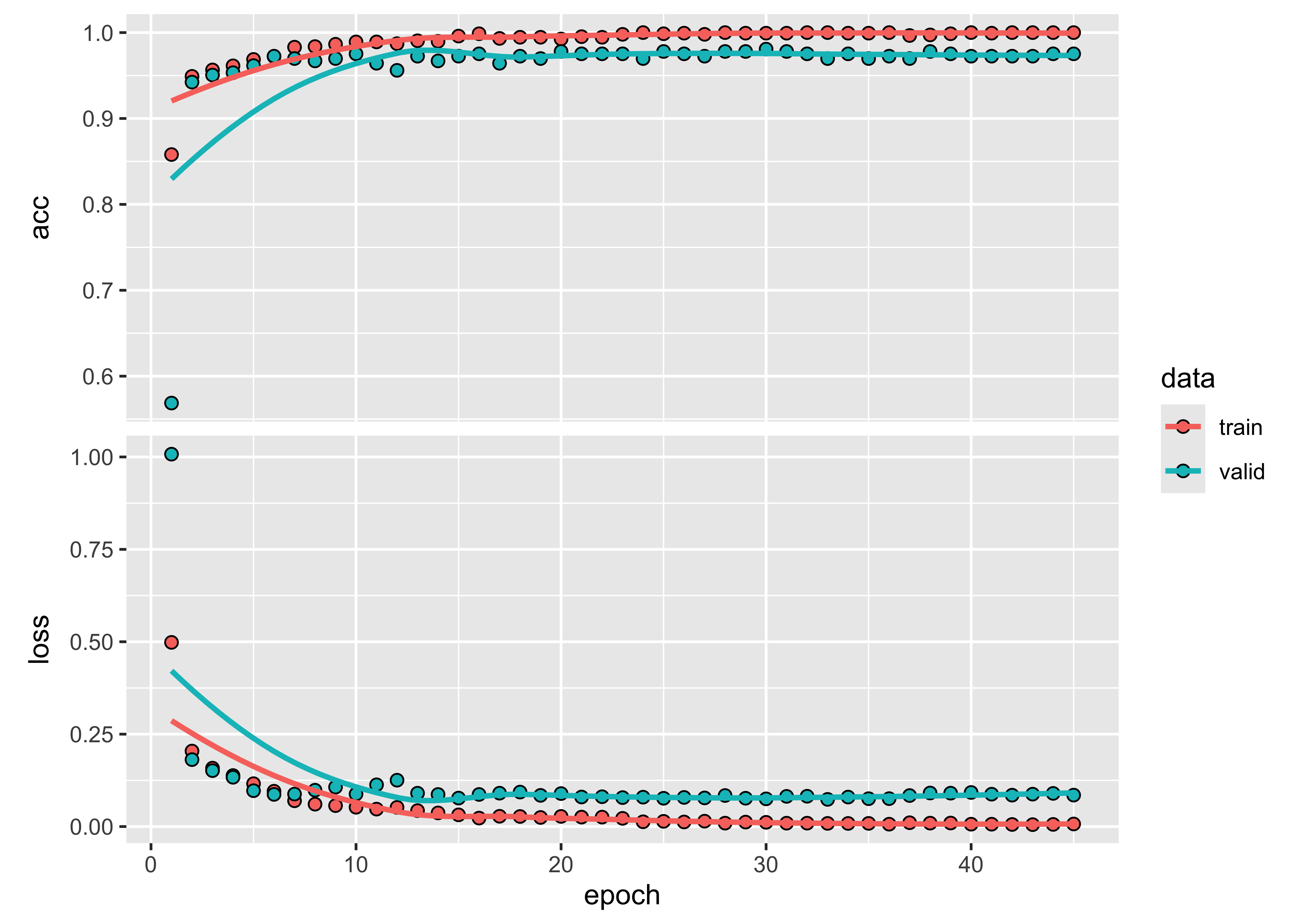

Figure 55: Training evolution of TempCNN model (Source: Authors).

Then, we classify a 16-year time series using the TempCNN model.

# Classify using TempCNN model and plot the result
class <- point_mt_mod13q1 |>
  sits_classify(tempcnn_model) |>
  plot(bands = c("NDVI", "EVI"))

Figure 56: Classification of time series using TempCNN (Source: Authors).

The result has important differences from the previous ones. The TempCNN model indicates the Soy_Cotton class as the most likely one in 2004. While this result is possibly wrong, it shows that the time series for 2004 is different from those of Forest and Pasture classes. One possible explanation is that there was forest degradation in 2004, leading to a signature that is a mix of forest and bare soil. In this case, including forest degradation samples could improve the training data. In our experience, TempCNN models are a reliable way of classifying image time series [60]. Recent work which compares different models also provides evidence that TempCNN models have satisfactory behavior, especially in the case of crop classes [61].

Residual 1D CNN networks (ResNet)

A residual 1D CNN network, also known as ResNet, is an extension of the standard 1D CNN architecture, adding residual connections between the layers. Residual connections allow the network to learn residual mappings, which are the difference between the input and output of a layer. By adding these residual connections, the network can learn to bypass specific layers and still capture essential features in the data.

The Residual Network (ResNet) for time series classification was proposed by Wang et al. [57], based on the idea of deep residual networks for 2D image recognition [62]. The ResNet architecture comprises 11 layers, with three blocks of three 1D CNN layers each (see Figure 57). Each block corresponds to a 1D CNN architecture. The output of each block is combined with a shortcut that links its output to its input, called a skip connection. The purpose of combining the input layer of each block with its output layer (after the convolutions) is to avoid the so-called “vanishing gradient problem”. This issue occurs in deep networks as the neural network’s weights are updated based on the partial derivative of the error function. If the gradient is too small, the weights will not be updated, stopping the training [63]. Skip connections aim to avoid vanishing gradients from occurring, allowing deep networks to be trained.

Figure 57: Structure of ResNet architecture (Source: Wang et al. (2017). Reproduction under fair use doctrine).

In sits, the Residual Network is implemented using sits_resnet(). The default parameters are those proposed by Wang et al. [57], as implemented by Fawaz et al. [64]. The first parameter is blocks, which controls the number of blocks and the size of filters in each block. By default, the model implements three blocks, the first with 64 filters and the others with 128. The parameter kernels controls the size of the kernels of the three layers inside each block. It is useful to experiment a bit with these kernel sizes in the case of satellite image time series. The default activation is “relu”, which is recommended in the literature to reduce the problem of vanishing gradients. The default optimizer is optim_adamw, available in package torchopt.

# Train using ResNet
resnet_model <- sits_train(
  samples_matogrosso_mod13q1,
  sits_resnet(
    blocks               = c(64, 128, 128),
    kernels              = c(7, 5, 3),
    epochs               = 100,
    batch_size           = 64,
    validation_split     = 0.2,
    verbose              = FALSE
  )
)
# Show training evolution
plot(resnet_model)

Figure 58: Training evolution of ResNet model (Source: Authors).

Then, we classify a 16-year time series using the ResNet model. The behavior of the ResNet model is similar to that of TempCNN, with more variability.

# Classify using DL model and plot the result
class <- point_mt_mod13q1 |>
  sits_classify(resnet_model) |>
  plot(bands = c("NDVI", "EVI"))

Figure 59: Classification of time series using ResNet (Source: Authors).

Attention-based models

Attention-based deep learning models are a class of models that use a mechanism inspired by human attention to focus on specific parts of input during processing. These models have been shown to be effective for various tasks such as machine translation, image captioning, and speech recognition.

The basic idea behind attention-based models is to allow the model to selectively focus on different input parts at different times. This can be done by introducing a mechanism that assigns weights to each element of the input, indicating the relative importance of that element to the current processing step. The model can then use them to compute a weighted sum of the input. The results capture the model’s attention on specific parts of the input.

Attention-based models have become one of the most used deep learning architectures for problems that involve sequential data inputs, e.g., text recognition and automatic translation. The general idea is that not all inputs are alike in applications such as language translation. Consider the English sentence “Look at all the lonely people”. A sound translation system needs to relate the words “look” and “people” as the key parts of this sentence to ensure such link is captured in the translation. A specific type of attention models, called transformers, enables the recognition of such complex relationships between input and output sequences [65].

The basic structure of transformers is the same as other neural network algorithms. They have an encoder that transforms textual input values into numerical vectors and a decoder that processes these vectors to provide suitable answers. The difference is how the values are handled internally. In an MLP, all inputs are treated equally at first; based on iterative matching of training and test data, the backpropagation technique feeds information back to the initial layers to identify the most suitable combination of inputs that produces the best output.

Convolutional nets (CNN) combine input values that are close in time (1D) or space (2D) to produce higher-level information that helps to distinguish the different components of the input data. For text recognition, the initial choice of deep learning studies was to use recurrent neural networks (RNN) that handle input sequences.

However, neither MLPs, CNNs, or RNNs have been able to capture the structure of complex inputs such as natural language. The success of transformer-based solutions accounts for substantial improvements in natural language processing.

The two main differences between transformer models and other algorithms are positional encoding and self-attention. Positional encoding assigns an index to each input value, ensuring that the relative locations of the inputs are maintained throughout the learning and processing phases. Self-attention compares every word in a sentence to every other word in the same sentence, including itself. In this way, it learns contextual information about the relation between the words. This conception has been validated in large language models such as BERT [66] and GPT-3 [67].

The application of attention-based models for satellite image time series analysis is proposed by Garnot et al. [68] and Russwurm and Körner [61]. A self-attention network can learn to focus on specific time steps and image features most relevant for distinguishing between different classes. The algorithm tries to identify which combination of individual temporal observations is most relevant to identify each class. For example, crop identification will use observations that capture the onset of the growing season, the date of maximum growth, and the end of the growing season. In the case of deforestation, the algorithm tries to identify the dates when the forest is being cut. Attention-based models are a means to identify events that characterize each land class.

The first model proposed by Garnot et al. is a full transformer-based model [68]. Considering that image time series classification is easier than natural language processing, Garnot et al. also propose a simplified version of the full transformer model [69]. This simpler model uses a reduced way to compute the attention matrix, reducing time for training and classification without loss of quality of the result.

In sits, the full transformer-based model proposed by Garnot et al. [68] is implemented using sits_tae(). The default parameters are those proposed by the authors. The default optimizer is the same optim_adamw, available in package torchopt.

# Train a machine learning model using TAE
tae_model <- sits_train(
  samples_matogrosso_mod13q1,
  sits_tae(
    epochs               = 150,
    batch_size           = 64,
    optimizer            = torchopt::optim_adamw,
    validation_split     = 0.2,
    verbose              = FALSE
  )
)
# Show training evolution
plot(tae_model)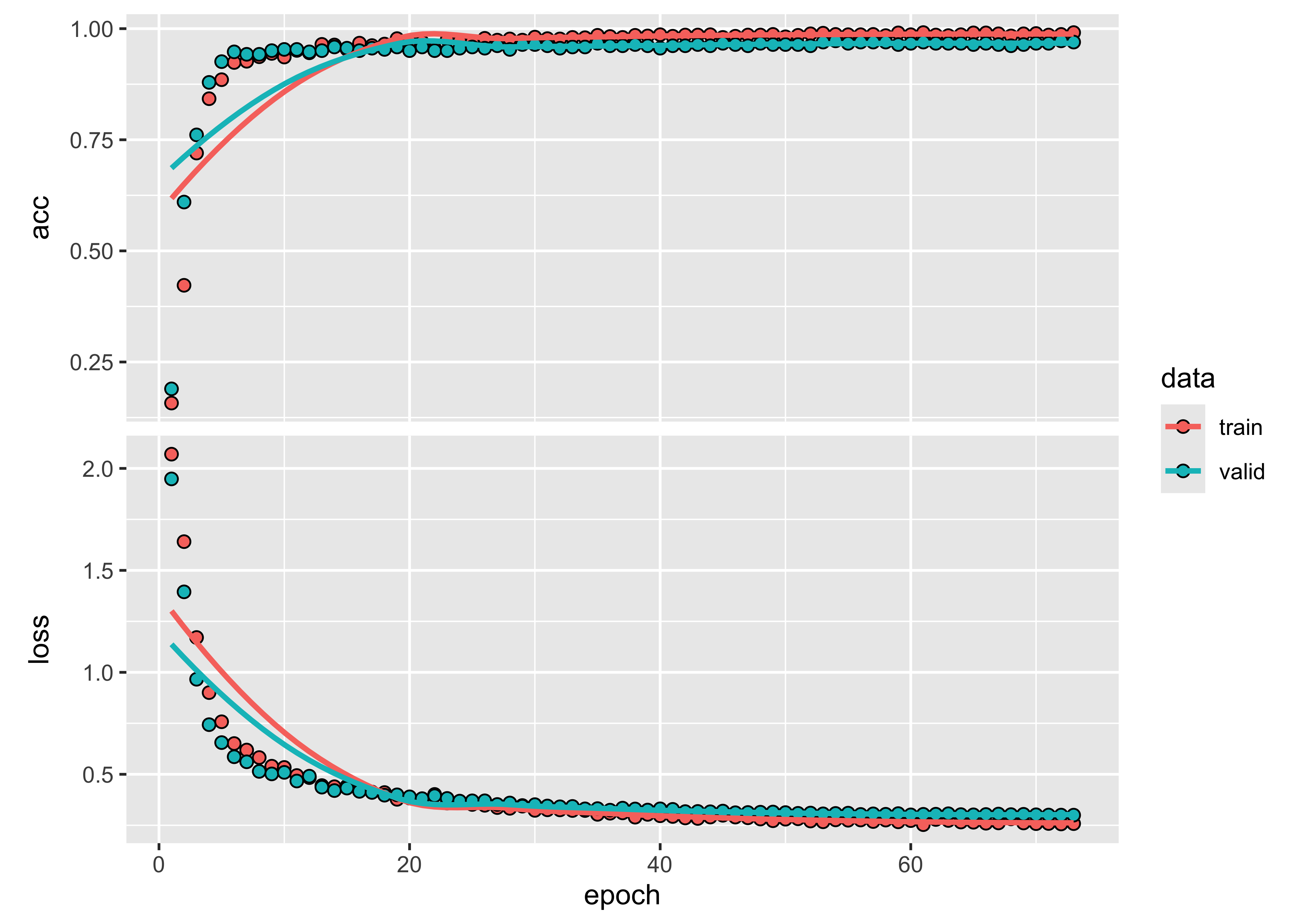

Figure 60: Training evolution of Temporal Self-Attention model (Source: Authors).

Then, we classify a 16-year time series using the TAE model.

# Classify using DL model and plot the result
class <- point_mt_mod13q1 |>
  sits_classify(tae_model) |>
  plot(bands = c("NDVI", "EVI"))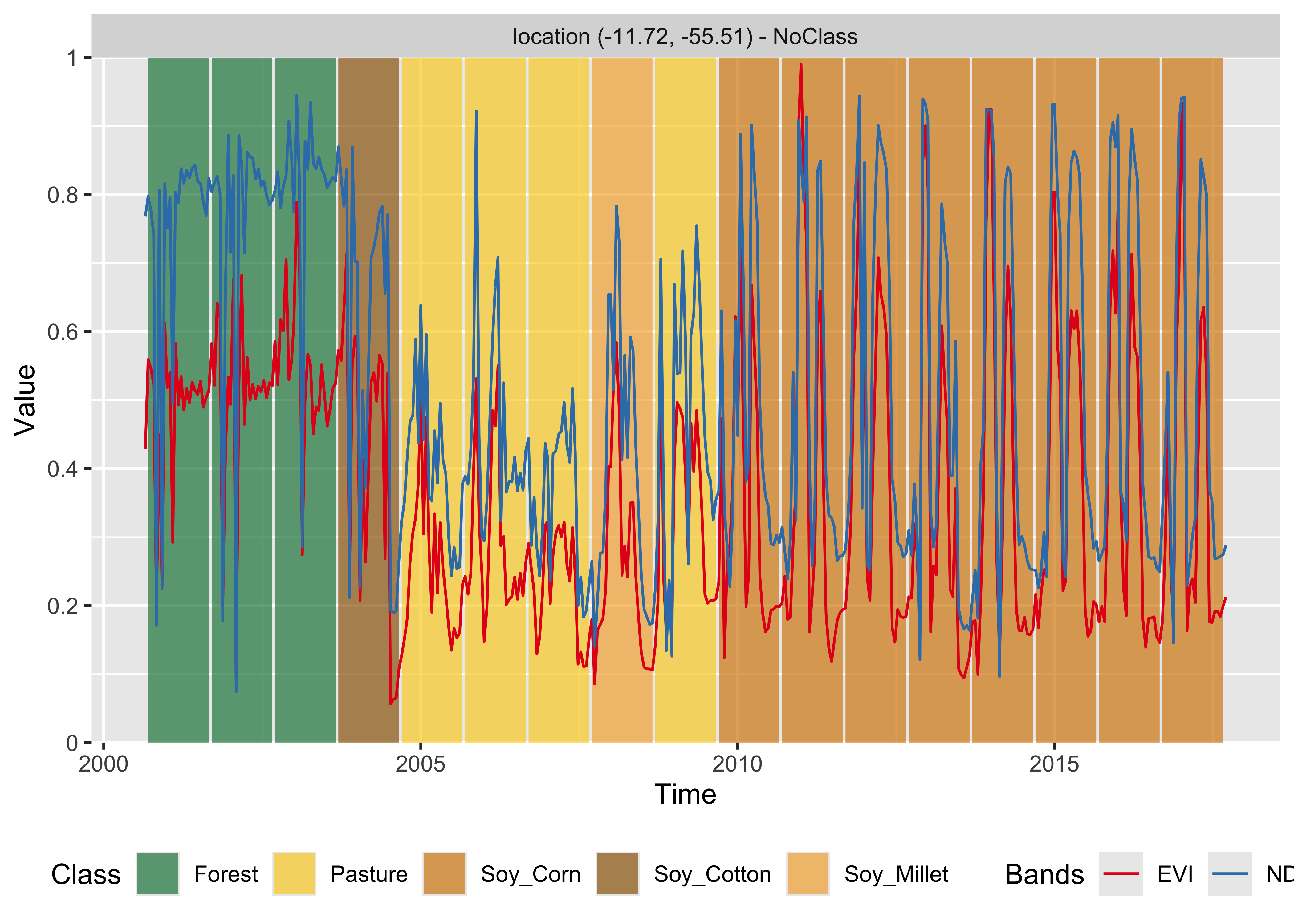

Figure 61: Classification of time series using TAE (Source: Authors).

Garnot and co-authors also proposed the Lightweight Temporal Self-Attention Encoder (LTAE) [69], which the authors claim can achieve high classification accuracy with fewer parameters compared to other neural network models. It is a good choice for applications where computational resources are limited. The sits_lighttae() function implements this algorithm. The default optimizer is optim_adamw, available in package torchopt. The most important parameter to be set is the learning rate lr. Values ranging from 0.001 to 0.005 should produce good results. See also the section below on model tuning.

# Train a machine learning model using TAE
ltae_model <- sits_train(
  samples_matogrosso_mod13q1,
  sits_lighttae(
    epochs = 150,
    batch_size = 64,
    optimizer = torchopt::optim_adamw,
    opt_hparams = list(lr = 0.001),
    validation_split = 0.2
  )
)
# Show training evolution
plot(ltae_model)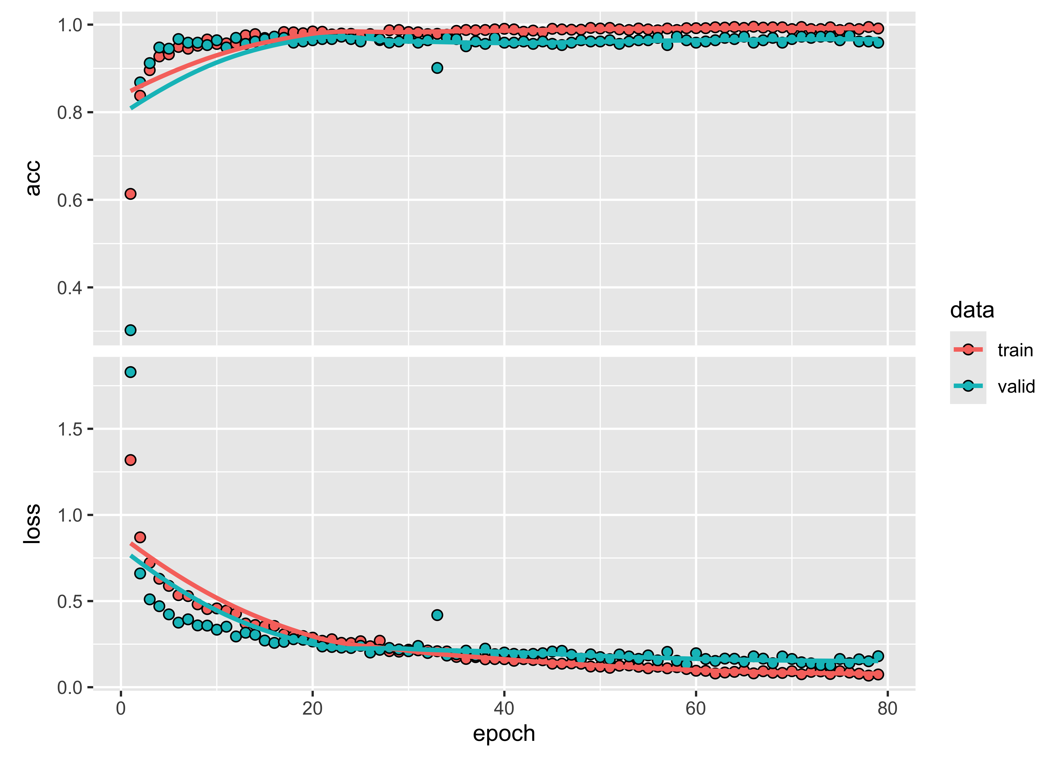

Figure 62: Training evolution of Lightweight Temporal Self-Attention model (Source: Authors).

Then, we classify a 16-year time series using the LightTAE model.

# Classify using DL model and plot the result
class <- point_mt_mod13q1 |>
  sits_classify(ltae_model) |>
  plot(bands = c("NDVI", "EVI"))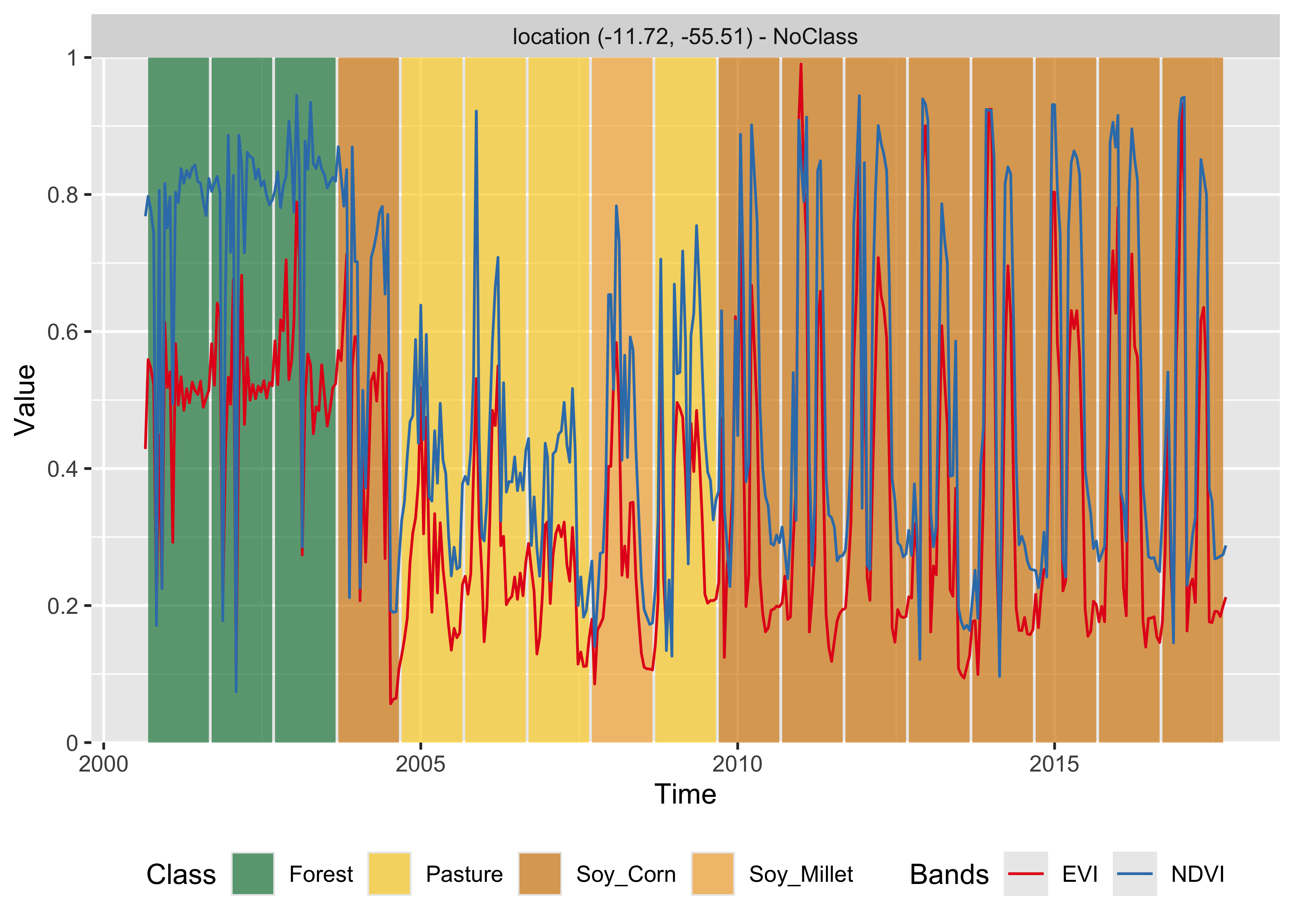

Figure 63: Classification of time series using LightTAE (Source: Authors).

The behaviour of both sits_tae() and sits_lighttae() is similar to that of sits_tempcnn(). It points out the possible need for more classes and training data to better represent the transition period between 2004 and 2010. One possibility is that the training data associated with the Pasture class is only consistent with the time series between the years 2005 to 2008. However, the transition from Forest to Pasture in 2004 and from Pasture to Agriculture in 2009-2010 is subject to uncertainty since the classifiers do not agree on the resulting classes. In general, deep learning temporal-aware models are more sensitive to class variability than random forest and extreme gradient boosters.

Deep learning model tuning

Model tuning is the process of selecting the best set of hyperparameters for a specific application. When using deep learning models for image classification, it is a highly recommended step to enable a better fit of the algorithm to the training data. Hyperparameters are parameters of the model that are not learned during training but instead are set prior to training and affect the behavior of the model during training. Examples include the learning rate, batch size, number of epochs, number of hidden layers, number of neurons in each layer, activation functions, regularization parameters, and optimization algorithms.

Deep learning model tuning involves selecting the best combination of hyperparameters that results in the optimal performance of the model on a given task. This is done by training and evaluating the model with different sets of hyperparameters to select the set that gives the best performance.

Deep learning algorithms try to find the optimal point representing the best value of the prediction function that, given an input \(X\) of data points, predicts the result \(Y\). In our case, \(X\) is a multidimensional time series, and \(Y\) is a vector of probabilities for the possible output classes. For complex situations, the best prediction function is time-consuming to estimate. For this reason, deep learning methods rely on gradient descent methods to speed up predictions and converge faster than an exhaustive search [70]. All gradient descent methods use an optimization algorithm adjusted with hyperparameters such as the learning and regularization rates [71]. The learning rate controls the numerical step of the gradient descent function, and the regularization rate controls model overfitting. Adjusting these values to an optimal setting requires using model tuning methods.

To reduce the learning curve, sits provides default values for all machine learning and deep learning methods, ensuring a reasonable baseline performance. However, refininig model hyperparameters might be necessary, especially for more complex models such as sits_lighttae() or sits_tempcnn(). To that end, the package provides the sits_tuning() function.

The most straightforward approach to model tuning is to run a grid search; this involves defining a range for each hyperparameter and then testing all possible combinations. This approach leads to a combinatorial explosion and thus is not recommended. Instead, Bergstra and Bengio propose randomly chosen trials [72]. Their paper shows that randomized trials are more efficient than grid search trials, selecting adequate hyperparameters at a fraction of the computational cost. The sits_tuning() function follows Bergstra and Bengio by using a random search on the chosen hyperparameters.

Since gradient descent plays a key role in deep learning model fitting, developing optimizers is an important topic of research [73]. Many optimizers have been proposed in the literature, and recent results are reviewed by Schmidt et al. [71]. The Adamw optimizer provides a good baseline and reliable performance for general deep learning applications [74].

Experiments with image time series show that other optimizers may have better performance for the specific problem of land classification. For this reason, the authors developed the torchopt R package, which includes several recently proposed optimizers, including Madgrad [75], and Yogi [76]. Using the sits_tuning() function allows testing these and other optimizers available in torch and torch_opt packages.

The sits_tuning() function takes the following parameters:

1. samples: Training dataset to be used by the model.
2. samples_validation: Optional dataset containing time series to be used for validation. If missing, the next parameter will be used.
3. validation_split: If samples_validation is not used, this parameter defines the proportion of time series in the training dataset to be used for validation (default is 20%).
4. ml_method(): Deep learning method (either sits_mlp(), sits_tempcnn(), sits_resnet(), sits_tae() or sits_lighttae()).
5. params: Defines the optimizer and its hyperparameters by calling sits_tuning_hparams(), as shown in the example below.
6. trials: Number of trials to run the random search.
7. multicores: Number of cores to be used for the procedure.
8. progress: Show a progress bar?

The sits_tuning_hparams() function inside sits_tuning() allows defining optimizers and their hyperparameters, including lr (learning rate), eps (controls numerical stability), and weight_decay (controls overfitting). The default values for eps and weight_decay in all sits deep learning functions are 1e-08 and 1e-06, respectively. The default lr for sits_lighttae() and sits_tempcnn() is 0.005, and for sits_tae() and sits_resnet() is 0.001.

Users have different ways to randomize the hyperparameters, including:

1. choice() (a list of options);
2. uniform (a uniform distribution);
3. randint (random integers from a uniform distribution);
4. normal(mean, sd) (normal distribution);
5. beta(shape1, shape2) (beta distribution);
6. loguniform(max, min) (loguniform distribution).

We suggest to use the log-uniform distribution to search over a wide range of values that span several orders of magnitude. This is common for hyperparameters like learning rates, which can vary from very small values (e.g., 0.0001) to larger values (e.g., 1.0) in a logarithmic manner. By default, sits_tuning() uses a loguniform distribution between 10^-2 and 10^-4 for the learning rate and the same distribution between 10^-2 and 10^-8 for the weight decay.

tuned <- sits_tuning(
  samples = samples_matogrosso_mod13q1,
  ml_method = sits_lighttae(),
  params = sits_tuning_hparams(
    optimizer = torch::optim_adamw,
    opt_hparams = list(
      lr = loguniform(10^-2, 10^-4),
      weight_decay = loguniform(10^-2, 10^-8)
    )
  ),
  trials = 40,
  multicores = 6,
  progress = FALSE
)

The result is a tibble with different values of accuracy, kappa, decision matrix, and hyperparameters. The best results obtain accuracy values between 0.978 and 0.970, as shown below. The best result is obtained by a learning rate of 0.0013 and a weight decay of 3.73e-07. The worst result has an accuracy of 0.891, which shows the importance of the tuning procedure.

# Obtain accuracy, kappa, lr, and weight decay for the 5 best results
# Hyperparameters are organized as a list
hparams_5 <- tuned[1:5, ]$opt_hparams
# Extract learning rate and weight decay from the list
lr_5 <- purrr::map_dbl(hparams_5, function(h) h$lr)
wd_5 <- purrr::map_dbl(hparams_5, function(h) h$weight_decay)

# Create a tibble to display the results
best_5 <- tibble::tibble(
  accuracy = tuned[1:5, ]$accuracy,
  kappa = tuned[1:5, ]$kappa,
  lr = lr_5,
  weight_decay = wd_5
)
# Print the best five combination of hyperparameters
best_5

#> # A tibble: 5 × 4
#>   accuracy kappa       lr weight_decay
#>      <dbl> <dbl>    <dbl>        <dbl>
#> 1    0.978 0.974 0.00136  0.000000373 
#> 2    0.975 0.970 0.00269  0.0000000861
#> 3    0.973 0.967 0.00162  0.00218     
#> 4    0.970 0.964 0.000378 0.00000868  
#> 5    0.970 0.964 0.00198  0.00000275

For large datasets, the tuning process is time-consuming. Despite this cost, it is recommended to achieve the best performance. In general, tuning hyperparameters for models such as sits_tempcnn() and sits_lighttae() will result in a slight performance improvement over the default parameters on overall accuracy. The performance gain will be stronger in the less well represented classes, where significant gains in producer’s and user’s accuracies are possible. When detecting change in less frequent classes, tuning can make a substantial difference in the results.

Considerations on model choice

The results should not be taken as an indication of which method performs better. The most crucial factor for achieving a good result is the quality of the training data [29]. Experience shows that classification quality depends on the training samples and how well the model matches these samples. For examples of ML for classifying large areas, please see the papers by the authors [5], [46], [77], [78].

In the specific case of satellite image time series, Russwurm et al. present a comparative study between seven deep neural networks for the classification of agricultural crops, using random forest as a baseline [61]. The data is composed of Sentinel-2 images over Britanny, France. Their results indicate a slight difference between the best model (attention-based transformer model) over TempCNN, ResNet, and random forest. Attention-based models obtain accuracy ranging from 80-81%, TempCNN gets 78-80%, and random forest obtains 78%. Based on this result and also on the authors’ experience, we make the following recommendations:

1. Random forest provides a good baseline for image time series classification and should be included in users’ assessments.

2. XGBoost is a worthy alternative to random forest. In principle, XGBoost is more sensitive to data variations at the cost of possible overfitting.

3. TempCNN is a reliable model with reasonable training time, which is close to the state-of-the-art in deep learning classifiers for image time series.

4. Attention-based models (TAE and LightTAE) can achieve the best overall performance with well-designed and balanced training sets and hyperparameter tuning.

5. The best means of improving classification performance is to provide an accurate and reliable training dataset. Each class should have enough samples to account for spatial and temporal variability.