Image classification in data cubes

This Chapter discusses how to classify data cubes by providing a step-by-step example. Our study area is the state of Rondonia, Brazil, which underwent substantial deforestation in the last decades. The objective of the case study is to detect deforested areas.
Data cube for case study
The examples of this chapter use a pre-built data cube of Sentinel-2 images, available in the package sitsdata. These images are from the SENTINEL-2-L2A collection in Microsoft Planetary Computer (MPC). The data consists of bands BO2, B8A, and B11, and indexes NDVI, EVI and NBR in a small area of \(1200 \times 1200\) pixels in the state of Rondonia. As explained in Chapter Earth observation data cubes, we must inform sits how to parse these file names to obtain tile, date, and band information. Image files are named according to the convention “satellite_ sensor_tile_band_date” (e.g., SENTINEL-2_MSI_20LKP_BO2_2020_06_04.tif) which is the default format in sits.
# Files are available in a local directory
data_dir <- system.file("extdata/Rondonia-20LMR/", package = "sitsdata")
# Read data cube
cube_20LMR <- sits_cube(
  source = "MPC",
  collection = "SENTINEL-2-L2A",
  data_dir = data_dir
)

# Plot the cube
plot(cube_20LMR, date = "2022-07-16", red = "B11", green = "B8A", blue = "B02")
Figure 63: Color composite image of the cube for date 2023-07-16 (Source: authors).
Training data for the case study
This case study uses the training data set samples_deforestation, available in package sitsdata. This data set consists of 6007 samples collected from Sentinel-2 images covering the state of Rondonia. There are nine classes: “Clear_Cut_Bare_Soil”, “Clear_Cut_Burned_Area”, “Mountainside_Forest”, “Forest”, “Riparian_Forest”, “Clear_Cut_Vegetation”, “Water”, “Wetland”, and “Seasonally_Flooded”. Each time series contains values from Sentinel-2/2A bands B02, B8A, B11, and indices NDVI, EVI and NBR from 2022-01-05 to 2022-12-23 in 16-day intervals. The samples are intended to detect deforestation events and have been collected by remote sensing experts using visual interpretation.
library(sitsdata)
# Obtain the samples
data("samples_deforestation")
# Show the contents of the samples
summary(samples_deforestation)
#> # A tibble: 9 × 3
#> label count prop
#> <chr> <int> <dbl>
#> 1 Clear_Cut_Bare_Soil 944 0.157
#> 2 Clear_Cut_Burned_Area 983 0.164
#> 3 Clear_Cut_Vegetation 603 0.100
#> 4 Forest 964 0.160
#> 5 Mountainside_Forest 211 0.0351
#> 6 Riparian_Forest 1247 0.208
#> 7 Seasonally_Flooded 731 0.122
#> 8 Water 109 0.0181
#> 9 Wetland 215 0.0358It is helpful to plot the basic patterns associated with the samples to understand the training set better. The function sits_patterns() uses a generalized additive model (GAM) to predict a smooth, idealized approximation to the time series associated with each class for all bands. Since the data cube used in the classification has three bands (B02, B8A, and B11) and three indexes (NDVI, EVI, NBR), we filter the samples for these bands and indexes before showing the patterns.
samples_deforestation |>
  sits_select(bands = c("NDVI", "EVI", "NBR")) |>
  sits_patterns() |>
  plot()
Figure 64: Patterns associated to the training samples (Source: Authors).
The patterns show different temporal responses for the selected classes. They match the typical behavior of deforestation in the Amazon. In most cases, the forest is cut at the start of the dry season (May/June). At the end of the dry season, some clear-cut areas are burned to clean the remains; this action is reflected in the steep fall of the response of NBR values of burned area samples after August. The areas where native trees have been cut but some vegatation remain (“Clear_Cut_Vegetation”) have values in the NBR band that increase during the period. This is a sign of mixed pixels, which combine forest remains with bare soil.
Training machine learning models
The next step is to train a machine learning model to illustrate CPU-based classification a random forest model and a tempCNN model. We build a Random Forest model using sits_train() and then plot the model to find out what are the most important variables for the model.
# Train model using Temporal CNN model
rfor_model <- sits_train(
  samples_deforestation,
  ml_method = sits_rfor()
)
plot(rfor_model)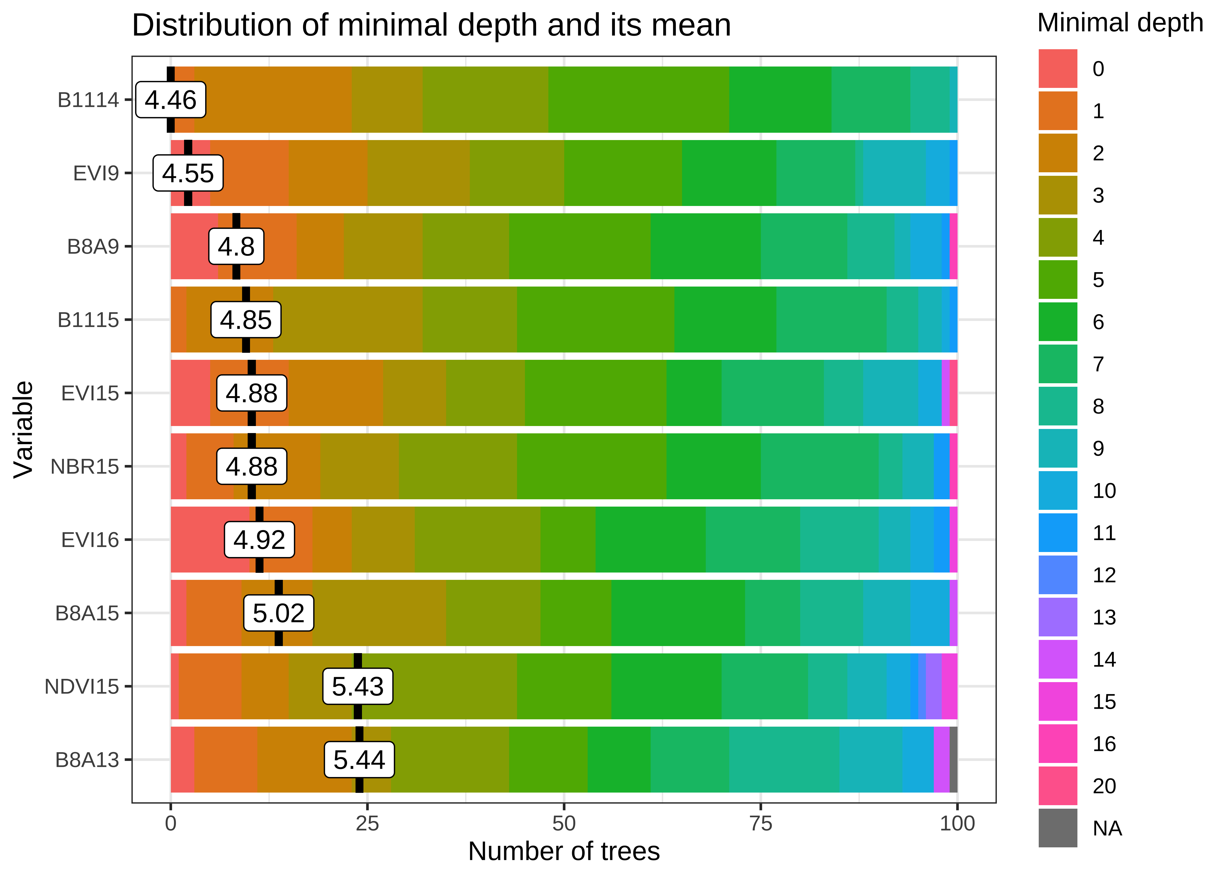
Figure 65: Most relevant variables of the Random Forest model (Source: Authors).
The figure shows that “B11” band values in date 15 (“2022-08-17”) is the most informative for the RF model, followed by “EVI” index values in date 9 (“2022-05-13”). These bands and dates represent inflection points in the image time series.
Classification of machine learning models in CPUs
The machine learning models available in sits (sits_rfor(), sits_svm() and sits_xgboost()) use CPU-based parallel processing, which is done internally by the package. The algorithms are adaptable; the only requirement for users is to inform the configuration of their machines. Details of CPU-based parallel processing in sits can be found in the Technical Annex.
To classify both data cubes and sets of time series, use sits_classify(), which uses parallel processing to speed up the performance, as described at the end of this Chapter. Its most relevant parameters are: (a) data, either a data cube or a set of time series; (b) ml_model, a trained model using one of the machine learning methods provided; (c) multicores, number of CPU cores that will be used for processing; (d) memsize, memory available for classification; (e) output_dir, directory where results will be stored; (f) version, for version control. To follow the processing steps, turn on the parameters verbose to print information and progress to get a progress bar. The classification result is a data cube with a set of probability layers, one for each output class. Each probability layer contains the model’s assessment of how likely each pixel belongs to the related class. The probability cube can be visualized with plot().
# Classify data cube to obtain a probability cube
cube_20LMR_probs <- sits_classify(
  data = cube_20LMR,
  ml_model = rfor_model,
  output_dir = "./tempdir/chp9",
  version = "rf-raster",
  multicores = 4,
  memsize = 16
)

plot(cube_20LMR_probs, labels = "Forest", palette = "YlGn")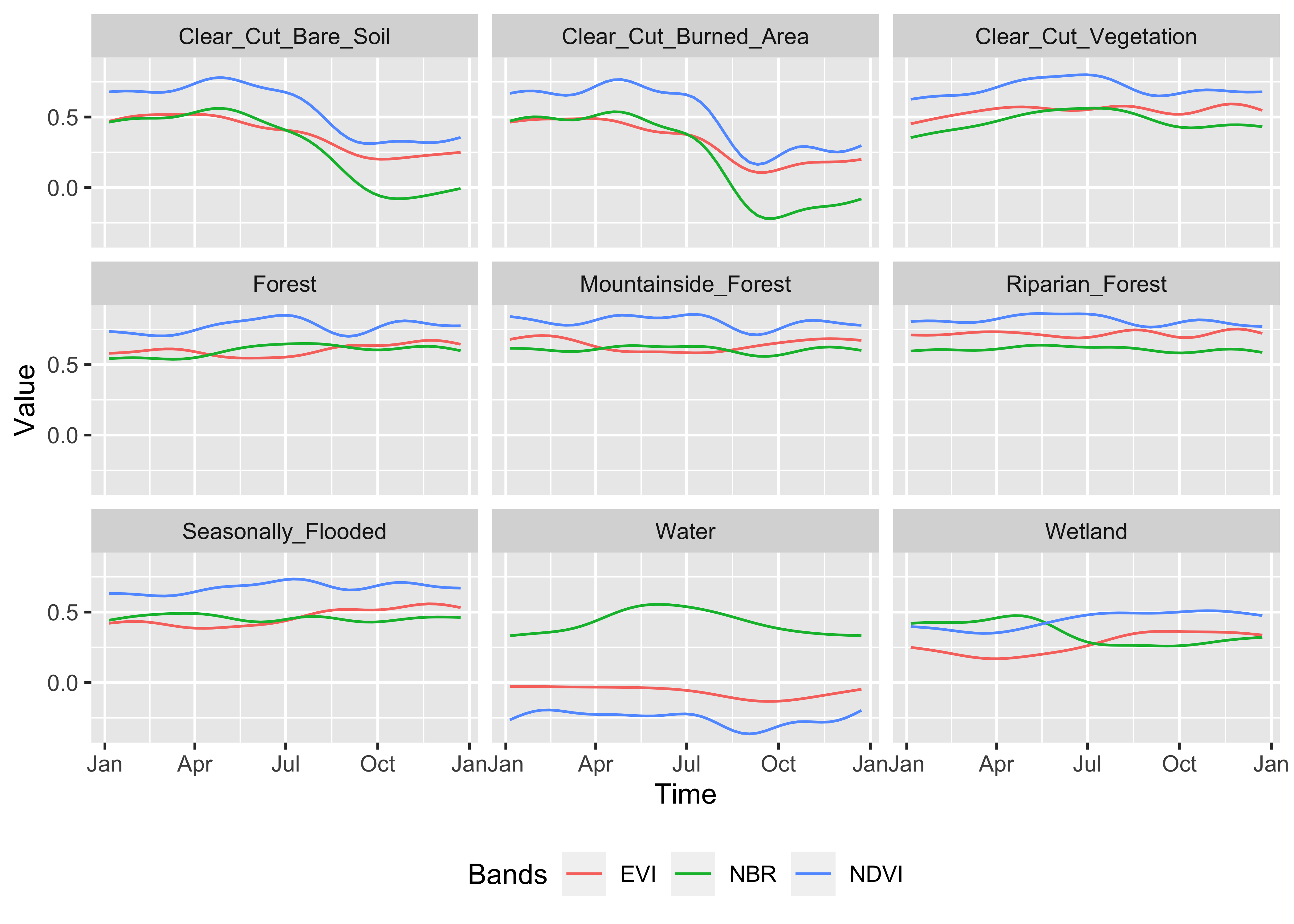
Figure 66: Probabilities for class Forest
The probability cube provides information on the output values of the algorithm for each class. Most probability maps contain outliers or misclassified pixels. The labeled map generated from the pixel-based time series classification method exhibits several misclassified pixels, which are small patches surrounded by a different class. This occurrence of outliers is a common issue that arises due to the inherent nature of this classification approach. Regardless of their resolution, mixed pixels are prevalent in images, and each class exhibits considerable data variability. As a result, these factors can lead to outliers that are more likely to be misclassified. To overcome this limitation, sits employs post-processing smoothing techniques that leverage the spatial context of the probability cubes to refine the results. These techniques will be discussed in the Chapter Bayesian smoothing for post-processing. In what follows, we will generate the smoothed cube to illustrate the procedure.
# Smoothen a  probability cube
cube_20LMR_bayes <- sits_smooth(
  cube = cube_20LMR_probs,
  output_dir = "./tempdir/chp9",
  version = "rf-raster",
  multicores = 4,
  memsize = 16
)
plot(cube_20LMR_bayes, labels = c("Forest", "Clear_Cut_Bare_Soil"), palette = "YlGn")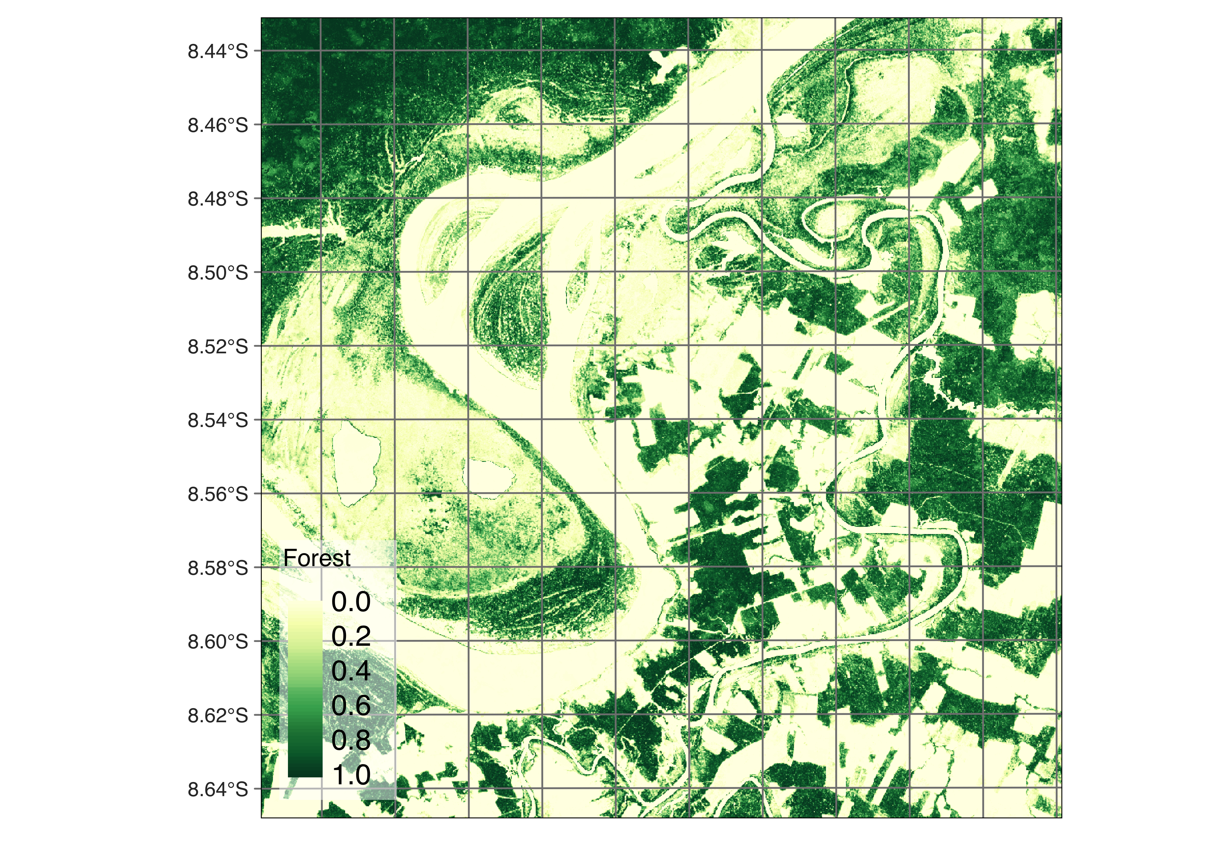
Figure 67: Smoothened probabilities for class Forest
In general, users should perform a post-processing smoothing after obtaining the probability maps in raster format. After the post-processing operation, we apply sits_label_classification() to obtain a map with the most likely class for each pixel. For each pixel, the sits_label_classification() function takes the label with highest probability and assigns it to the resulting map. The output is a labelled map with classes. In addition, the function will remove outliers using a modal filter after if the clean parameter is set to TRUE (default value). For each pixel, the modal filter scans a neighborhood defined by window_size (default = 3) and assigns such pixel to the most frequent label inside the window.
# Generate a thematic map
cube_20LMR_class <- sits_label_classification(
  cube = cube_20LMR_bayes,
  clean = TRUE,
  window_size = 3L,
  multicores = 4,
  memsize = 12,
  output_dir = "./tempdir/chp9",
  version = "rf-raster"
)

# Plot the thematic map
plot(cube_20LMR_class,
  tmap_options =
    list("scale" = 0.6)
)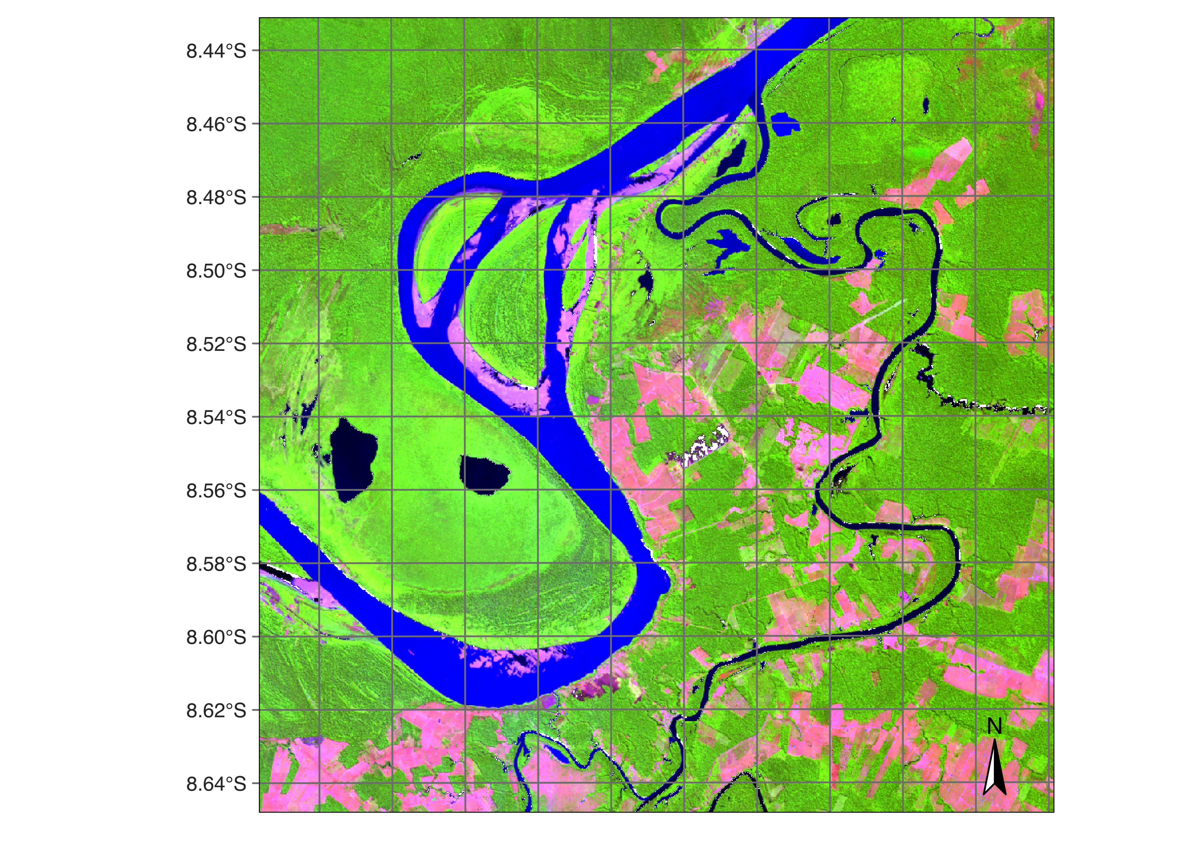
Figure 68: Final map of deforestation obtained by random forest model(Source: Authors).
Training and running deep learning models
The next examples shows how to run deep learning models in sits. This model will show how to run deep learning methods in GPUs if available. The case study uses the Temporal CNN model [58], which is described in ChapterMachine learning for data cubes. We first show the need for model tuning, before applying the model for data cube classification.
Deep learning model tuning
In the example, we use sits_tuning() to find good hyperparameters to train the sits_tempcnn() algorithm for the Rondonia training data set. The hyperparameters for the sits_tempcnn() method include the size of the layers, convolution kernels, dropout rates, learning rate and weight decay. Please refer to description of the Temporal CNN algorithm in Chapter Machine learning for data cubes
tuned_tempcnn <- sits_tuning(
  samples = samples_deforestation,
  ml_method = sits_tempcnn(),
  params = sits_tuning_hparams(
    cnn_layers = choice(c(256, 256, 256), c(128, 128, 128), c(64, 64, 64)),
    cnn_kernels = choice(c(3, 3, 3), c(5, 5, 5), c(7, 7, 7)),
    cnn_dropout_rates = choice(
      c(0.15, 0.15, 0.15), c(0.2, 0.2, 0.2),
      c(0.3, 0.3, 0.3), c(0.4, 0.4, 0.4)
    ),
    optimizer = torchopt::optim_adamw,
    opt_hparams = list(
      lr = loguniform(10^-2, 10^-4),
      weight_decay = loguniform(10^-2, 10^-8)
    )
  ),
  trials = 50,
  multicores = 4
)
The result of sits_tuning() is tibble with different values of accuracy, kappa, decision matrix, and hyperparameters. The five best results obtain accuracy values between 0.939 and 0.908, as shown below. The best result is obtained by a learning rate of 3.76e-04 and a weight decay of 1.5e-04, and three CNN layers of size 256, kernel size of 5, and dropout rates of 0.2.
# Obtain accuracy, kappa, cnn_layers, cnn_kernels, and cnn_dropout_rates the best result
cnn_params <- tuned_tempcnn[1, c("accuracy", "kappa", "cnn_layers", "cnn_kernels", "cnn_dropout_rates"), ]
# Learning rates and weight decay are organized as a list
hparams_best <- tuned_tempcnn[1, ]$opt_hparams[[1]]
# Extract learning rate and weight decay
lr_wd <- tibble::tibble(
  lr_best = hparams_best$lr,
  wd_best = hparams_best$weight_decay
)
# Print the best parameters
dplyr::bind_cols(cnn_params, lr_wd)
#> # A tibble: 1 × 7
#> accuracy kappa cnn_layers cnn_kernels cnn_dropout_rates lr_best wd_best
#> <dbl> <dbl> <chr> <chr> <chr> <dbl> <dbl>
#> 1 0.939 0.929 c(256, 256, 256) c(5, 5, 5) c(0.2, 0.2, 0.2) 0.000376 0.000153Classification in GPUs using parallel processing
Deep learning time series classification methods in sits, which include sits_tempcnn(), sits_mlp(), sits_resnet(), sits_lightae() and sits_tae(), are written using the torch package, which is an adaptation of pyTorch to the R environment. These algorithms can use a CUDA-compatible NVDIA GPU which has been properly configured. Please refer to the torch installation guide for details. If no GPU is available, these algorithms will run on regular CPUs, using the same paralellization methods as traditional machine learning methods. Typically, there is a 10-fold performance increase when running torch based methods in GPUs relative to their processing time in GPU.
To illustrate the use of GPUs, we take the same data cube and training data used in the previous examples and use a Temporal CNN method. The first step is to obtain a deep learning model using the hyperparameters produced by the tuning procedure shown earlier. We run
tcnn_model <- sits_train(
  samples_deforestation,
  sits_tempcnn(
    cnn_layers = c(256, 256, 256),
    cnn_kernels = c(5, 5, 5),
    cnn_dropout_rates = c(0.2, 0.2, 0.2),
    opt_hparams = list(
      lr = 0.000376,
      weight_decay = 0.000153
    )
  )
)
After training the model, we classify the data cube. If a GPU is available, users need to provide the additional parameter gpu_memory to the sits_classify() function. This information will be used by sits to optimize access to the GPU and speed up processing.
cube_20LMR_probs_tcnn <- sits_classify(
  cube_20LMR,
  ml_model = tcnn_model,
  output_dir = "./tempdir/chp9",
  version = "tcnn-raster",
  gpu_memory = 16,
  multicores = 6,
  memsize = 24
)
After classification, we can smooth the probability cube and then label the resulting smoothed probabilities to obtain a classified map.
# Smoothen the probability map
cube_20LMR_bayes_tcnn <- sits_smooth(
  cube_20LMR_probs_tcnn,
  output_dir = "./tempdir/chp9",
  version = "tcnn-raster",
  multicores = 6,
  memsize = 24
)
# Obtain the final labelled map
cube_20LMR_class_tcnn <- sits_label_classification(
  cube_20LMR_bayes_tcnn,
  output_dir = "./tempdir/chp9",
  version = "tcnn-raster",
  multicores = 6,
  memsize = 24
)
# plot the final classification map
plot(cube_20LMR_class_tcnn,
  tmap_options = list("scale" = 0.6)
)
Figure 69: Final map of deforestation obtained using TempCNN model (Source: Authors).
Map reclassification
Reclassification of a remote sensing map refers to changing the classes assigned to different pixels in the image. The purpose of reclassification is to modify the information contained in the image to better suit a specific use case. In sits, reclassification involves assigning new classes to pixels based on additional information from a reference map. Users define rules according to the desired outcome. These rules are then applied to the classified map. The result is a new map with updated classes.
To illustrate the reclassification in sits, we take a classified data cube stored in the sitsdata package. As discussed in Chapter Earth observation data cubes, sits can create a data cube from a classified image file. Users need to provide the original data source and collection, the directory where data is stored (data_dir), the information on how to retrieve data cube parameters from file names (parse_info), and the labels used in the classification.
# Open classification map
data_dir <- system.file("extdata/Rondonia-Class", package = "sitsdata")
ro_class <- sits_cube(
  source = "MPC",
  collection = "SENTINEL-2-L2A",
  data_dir = data_dir,
  parse_info = c(
    "satellite", "sensor", "tile", "start_date", "end_date",
    "band", "version"
  ),
  bands = "class",
  labels = c(
    "1" = "Water", "2" = "Clear_Cut_Burned_Area",
    "3" = "Clear_Cut_Bare_Soil",
    "4" = "Clear_Cut_Vegetation",
    "5" = "Forest",
    "6" = "Bare_Soil",
    "7" = "Wetland"
  )
)

plot(ro_class,
  tmap_options = list("scale" = 0.6)
)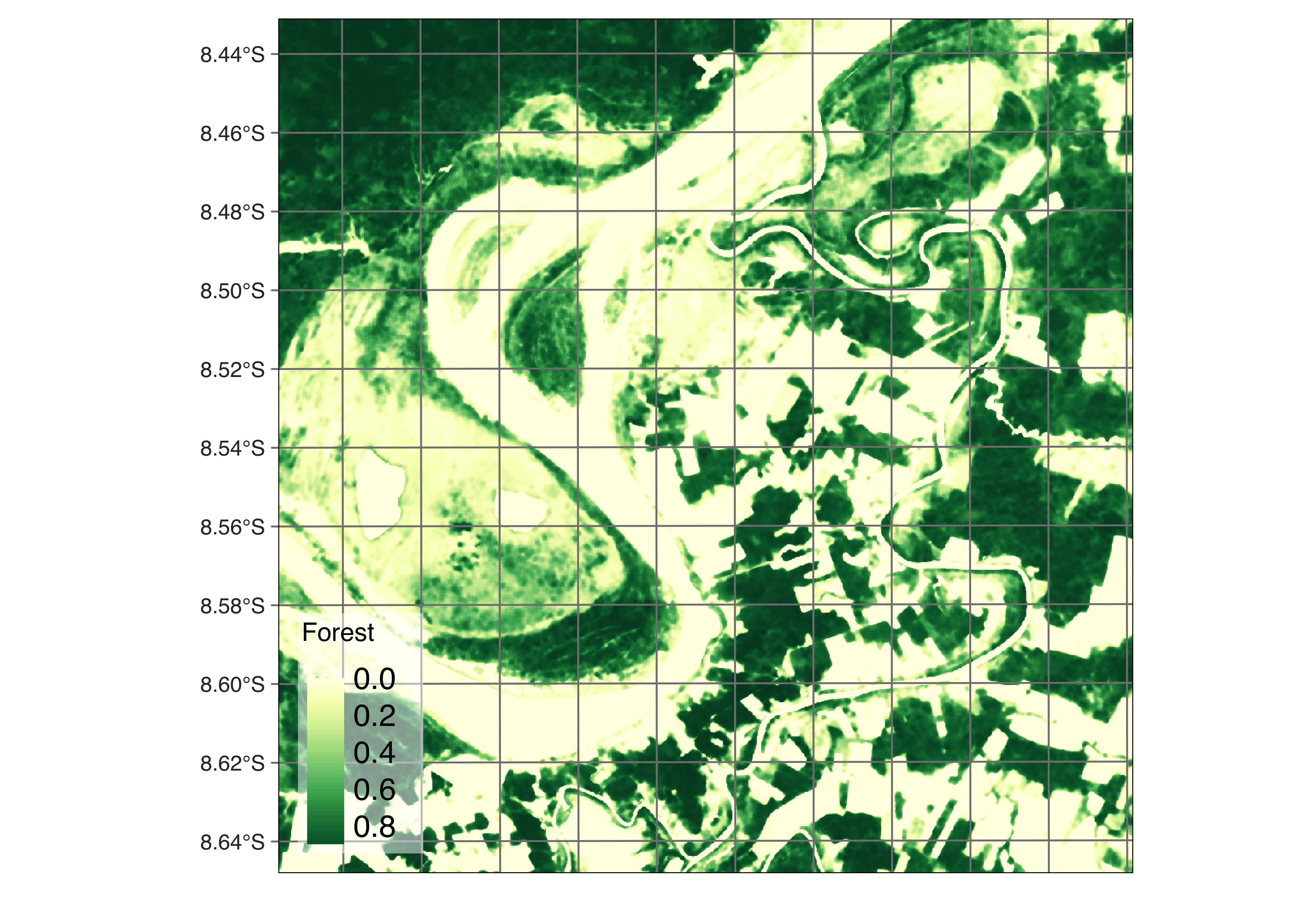
Figure 70: Original classification map (Source: Authors).
The above map shows the total extent of deforestation by clear cuts estimated by the sits random forest algorithm in an area in Rondonia, Brazil, based on a time series of Sentinel-2 images for the period 2020-06-04 to 2021-08-26. Suppose we want to estimate the deforestation that occurred from June 2020 to August 2021. We need a reference map containing information on forest cuts before 2020.
In this example, we use as a reference the PRODES deforestation map of Amazonia created by Brazil’s National Institute for Space Research (INPE). This map is produced by visual interpretation. PRODES measures deforestation every year, starting from August of one year to July of the following year. It contains classes that represent the natural world (Forest, Water, NonForest, and NonForest2) and classes that capture the yearly deforestation increments. These classes are named “dYYYY” and “rYYYY”; the first refers to deforestation in a given year (e.g., “d2008” for deforestation for August 2007 to July 2008); the second to places where the satellite data is not sufficient to determine the land class (e.g., “r2010” for 2010). This map is available on package sitsdata, as shown below.
data_dir <- system.file("extdata/PRODES", package = "sitsdata")
prodes2021 <- sits_cube(
  source = "USGS",
  collection = "LANDSAT-C2L2-SR",
  data_dir = data_dir,
  parse_info = c(
    "product", "sensor", "tile", "start_date", "end_date",
    "band", "version"
  ),
  bands = "class",
  version = "v20220606",
  labels = c(
    "1" = "Forest", "2" = "Water", "3" = "NonForest",
    "4" = "NonForest2", "6" = "d2007", "7" = "d2008",
    "8" = "d2009", "9" = "d2010", "10" = "d2011",
    "11" = "d2012", "12" = "d2013", "13" = "d2014",
    "14" = "d2015", "15" = "d2016", "16" = "d2017",
    "17" = "d2018", "18" = "r2010", "19" = "r2011",
    "20" = "r2012", "21" = "r2013", "22" = "r2014",
    "23" = "r2015", "24" = "r2016", "25" = "r2017",
    "26" = "r2018", "27" = "d2019", "28" = "r2019",
    "29" = "d2020", "31" = "r2020", "32" = "Clouds2021",
    "33" = "d2021", "34" = "r2021"
  )
)
Since the labels of the deforestation map are specialized and are not part of the default sits color table, we define a legend for better visualization of the different deforestation classes.
# Use the RColorBrewer palette "YlOrBr" for the deforestation years
colors <- grDevices::hcl.colors(n = 15, palette = "YlOrBr")
# Define the legend for the deforestation map
def_legend <- c(
  "Forest" = "forestgreen", "Water" = "dodgerblue3",
  "NonForest" = "bisque2", "NonForest2" = "bisque2",
  "d2007" = colors[1], "d2008" = colors[2],
  "d2009" = colors[3], "d2010" = colors[4],
  "d2011" = colors[5], "d2012" = colors[6],
  "d2013" = colors[7], "d2014" = colors[8],
  "d2015" = colors[9], "d2016" = colors[10],
  "d2017" = colors[11], "d2018" = colors[12],
  "d2019" = colors[13], "d2020" = colors[14],
  "d2021" = colors[15], "r2010" = "lightcyan",
  "r2011" = "lightcyan", "r2012" = "lightcyan",
  "r2013" = "lightcyan", "r2014" = "lightcyan",
  "r2015" = "lightcyan", "r2016" = "lightcyan",
  "r2017" = "lightcyan", "r2018" = "lightcyan",
  "r2019" = "lightcyan", "r2020" = "lightcyan",
  "r2021" = "lightcyan", "Clouds2021" = "lightblue2"
)
Using this new legend, we can visualize the PRODES deforestation map.
sits_view(prodes2021, legend = def_legend)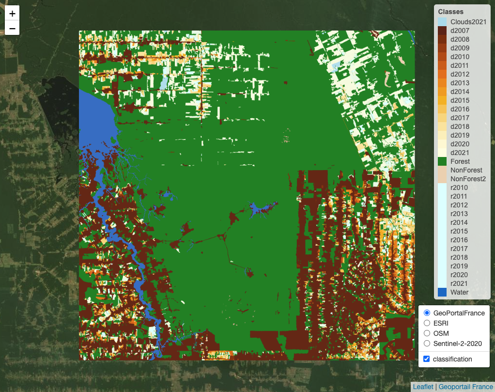
Figure 71: Deforestation map produced by PRODES.
Taking the PRODES map as our reference, we can include new labels in the classified map produced by sits using sits_reclassify(). The new class name Defor_2020 will be applied to all pixels that PRODES considers that have been deforested before July 2020. We also include a Non_Forest class to include all pixels that PRODES takes as not covered by native vegetation, such as wetlands and rocky areas. The PRODES classes will be used as a mask over the sits deforestation map.
The sits_reclassify() operation requires the parameters: (a) cube, the classified data cube whose pixels will be reclassified; (b) mask, the reference data cube used as a mask; (c) rules, a named list. The names of the rules list will be the new label. Each new label is associated with a mask vector that includes the labels of the reference map that will be joined. sits_reclassify() then compares the original and reference map pixel by pixel. For each pixel of the reference map whose labels are in one of the rules, the algorithm relabels the original map. The result will be a reclassified map with the original labels plus the new labels that have been masked using the reference map.
# Reclassify cube
ro_def_2021 <- sits_reclassify(
  cube = ro_class,
  mask = prodes2021,
  rules = list(
    "Non_Forest" = mask %in% c("NonForest", "NonForest2"),
    "Deforestation_Mask" = mask %in% c(
      "d2007", "d2008", "d2009",
      "d2010", "d2011", "d2012",
      "d2013", "d2014", "d2015",
      "d2016", "d2017", "d2018",
      "d2019", "d2020",
      "r2010", "r2011", "r2012",
      "r2013", "r2014", "r2015",
      "r2016", "r2017", "r2018",
      "r2019", "r2020", "r2021"
    ),
    "Water" = mask == "Water"
  ),
  memsize = 8,
  multicores = 2,
  output_dir = "./tempdir/chp9",
  version = "reclass"
)

# Plot the reclassified map
plot(ro_def_2021,
  tmap_options = list("scale" = 0.6)
)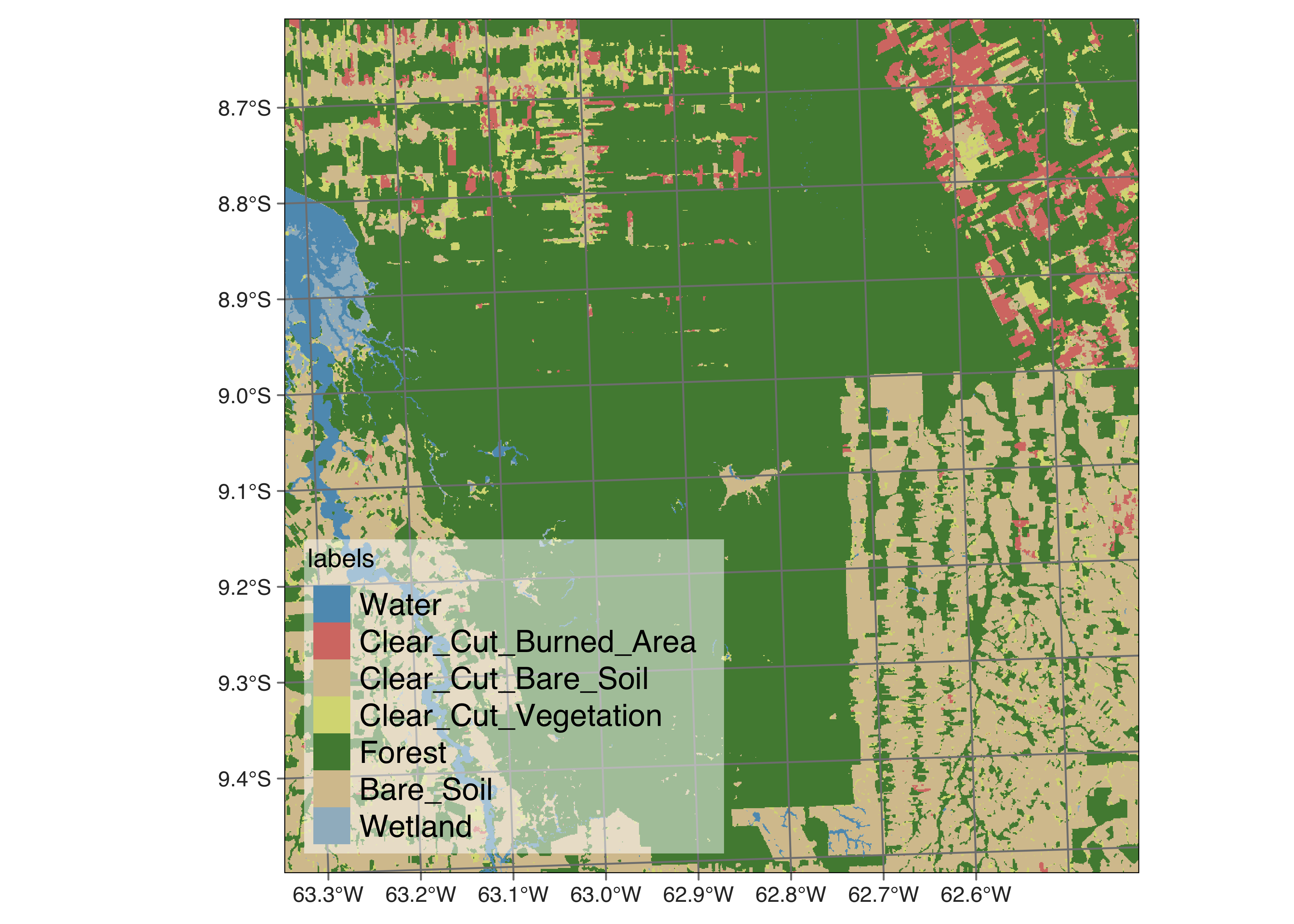
Figure 72: Deforestation map by sits masked by PRODES map (Source: Authors).
The reclassified map has been split into deforestation before mid-2020 (using the PRODES map) and the areas classified by sits that are taken as being deforested from mid-2020 to mid-2021. This allows the experts to measure how much deforestation occurred in this period according to sits and compare the result with the PRODES map.
The sits_reclassify() function is not restricted to comparing deforestation maps. It can be used in any case that requires masking of a result based on a reference map.