1 Introduction to `sits`

Why work with satellite image time series?

Satellite images are the most comprehensive source of data about our environment. Covering a large area of the Earth’s surface, images allow researchers to study regional and global changes. Sensors capture data in multiple spectral bands to measure the physical, chemical, and biological properties of the Earth’s surface. By observing the same location multiple times, satellites provide data on changes in the environment and survey areas that are difficult to observe from the ground. Given its unique features, images offer essential information for many applications, including deforestation, crop production, food security, urban footprints, water scarcity, and land degradation.

A time series is a set of data points collected at regular intervals over time. Time series data is used to analyze trends, patterns, and changes. Satellite image time series refer to time series obtained from a collection of images captured by a satellite over a period of time, typically months or years. Using time series, experts improve their understanding of ecological patterns and processes. Instead of selecting individual images from specific dates and comparing them, researchers track change continuously [1].

Time-first, space-later

“Time-first, space-later” is a concept in satellite image classification that takes time series analysis as the first step for analyzing remote sensing data, with spatial information being considered after all time series are classified. The time-first part brings a better understanding of changes in landscapes. Detecting and tracking seasonal and long-term trends becomes feasible, as well as identifying anomalous events or patterns in the data, such as wildfires, floods, or droughts. Each pixel in a data cube is treated as a time series, using information available in the temporal instances of the case. Time series classification is pixel-based, producing a set of labelled pixels. This result is then used as input to the space-later part of the method. In this phase, a Bayesian smoothing algorithm that considers the spatial neighbourhood of each pixel improves the results of pixel-based classification.

How `sits` works

The sits package uses satellite image time series for land classification, using a time-first, space-later approach. In the data preparation part, collections of big Earth observation images are organized as data cubes. Each spatial location of a data cube is associated with a time series. Locations with known labels train a machine learning algorithm, which classifies all time series of a data cube, as shown in Figure 1.

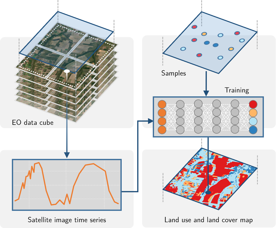
Figure 1.1: Using time series for land classification (source: authors).

The package provides tools for analysis, visualization, and classification of satellite image time series. Users follow a typical workflow:

Select an analysis-ready data image collection on cloud providers such as AWS, Microsoft Planetary Computer, Digital Earth Africa, or Brazil Data Cube.
Build a regular data cube using the chosen image collection.
Obtain new bands and indices with operations on data cubes.
Extract time series samples from the data cube to be used as training data.
Perform quality control and filtering on the time series samples.
Train a machine learning model using the time series samples.
Classify the data cube using the model to get class probabilities for each pixel.
Post-process the probability cube to remove outliers.
Produce a labeled map from the post-processed probability cube.
Evaluate the accuracy of the classification using best practices.

Each workflow step corresponds to a function of the sits API, as shown in the table and figure below. These functions have convenient default parameters and behaviors. A single function builds machine learning (ML) models. The classification function processes big data cubes with efficient parallel processing. Since the sits API is simple to learn, users can achieve good results without in-depth knowledge about machine learning and parallel processing.

In this book, we distinguish between the concepts of “class” and “label”. A class denotes a group of spatial objects that share similar land cover and land use, such as urban areas, forests, water bodies, or agricultural fields. Classes are defined based on the specific application or study being conducted, and they help to analyse the vast amount of data obtained from remote sensing imagery. A label is the assignment or identification given to a specific feature or object within an image. Labels are markers that indicate to which class a particular pixel, segment, or object belongs. Labels are essential for supervised classification methods, where a training dataset with known labels is used to train a machine learning algorithm to recognize and classify new, unlabelled data. Thus, a “class” represents the overall category or group of features, while a “label” refers to the specific assignment of a class to a particular feature or object within an image.

Table 1.1: The sits API workflow for land classification
API_function	Inputs	Output
sits_cube()	ARD image collection	Irregular data cube
sits_regularize()	Irregular data cube	Regular data cube
sits_apply()	Regular data cube	Regular data cube with new bands and indices
sits_get_data()	Data cube and sample locations	Time series
sits_train()	Time series and ML method	ML classification model
sits_classify()	ML classification model and regular data cube	Probability cube
sits_smooth()	Probability cube	Post-processed probability cube
sits_label_classification()	Post-processed probability cube	Classified map
sits_accuracy()	Classified map and validation samples	Accuracy assessment

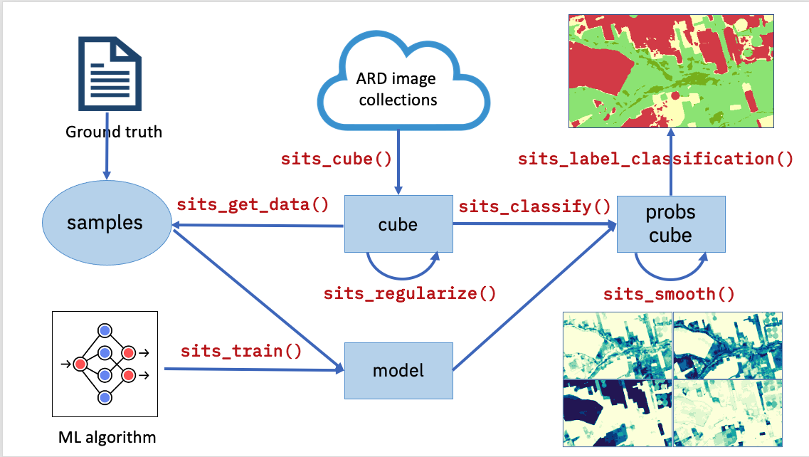
Figure 1.2: Main functions of the sits API (source: authors).

Creating a Data Cube

There are two kinds of data cubes in sits: (a) irregular data cubes generated by selecting image collections on cloud providers such as AWS and Planetary Computer; (b) regular data cubes with images fully covering a chosen area, where each image has the same spectral bands and spatial resolution, and images follow a set of adjacent and regular time intervals. Machine learning applications need regular data cubes. Please refer to Chapter Earth observation data cubes for further details.

The first steps in using sits are: (a) select an analysis-ready data image collection available in a cloud provider or stored locally using sits_cube(); (b) if the collection is not regular, use sits_regularize() to build a regular data cube.

This section shows how to build a data cube from local images already organized as a regular data cube. The data cube is composed of MODIS MOD13Q1 images for the Sinop region in Mato Grosso, Brazil. All images have indexes NDVI and EVI covering a one-year period from 2013-09-14 to 2014-08-29 (we use “year-month-day” for dates). There are 23 time instances, each covering a 16-day period. The data is available in the R package sitsdata.

To build a data cube from local files, users must provide information about the original source from which the data was obtained. In this case, sits_cube() needs the parameters:

source, the cloud provider from where the data has been obtained (in this case, the Brazil Data Cube “BDC”);
collection, the collection of the cloud provider from where the images have been extracted. In this case, data comes from the MOD13Q1 collection 6;
data_dir, the local directory where the image files are stored;
parse_info, a vector of strings stating how file names store information on “tile”, “band”, and “date”. In this case, local images are stored in files like TERRA_MODIS_012010_EVI_2014-07-28.tif. This file represents tile 012010, band EVI, and date 2014-07-28.

# Create a data cube object based on the information about the files
sinop <- sits_cube(
  source = "BDC",
  collection = "MOD13Q1-6",
  data_dir = system.file("extdata/sinop", package = "sitsdata"),
  parse_info = c("X1", "X2", "tile", "band", "date")
)

# Plot the NDVI for the first date (2013-09-14)
plot(sinop,
  band = "NDVI",
  dates = "2013-09-14",
  palette = "RdYlGn"
)

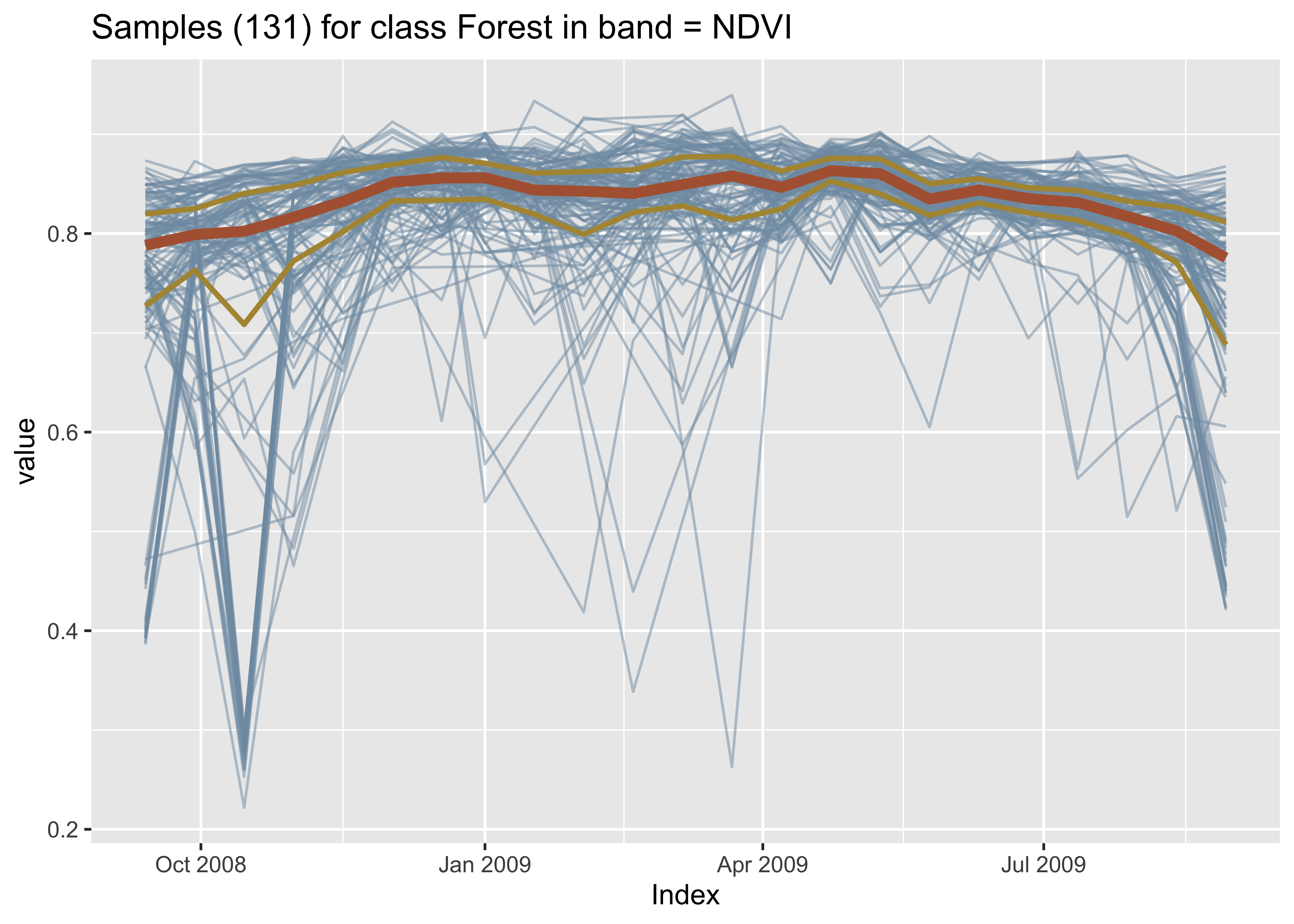
Figure 1.3: Color composite image MODIS cube for 2013-09-14 (red = EVI, green = NDVI, blue = EVI).

The aim of the parse_info parameter is to extract tile, band and date information from the file name. Given the large variation in image file names generated by different produces, it includes designators such as X1 and X2; these are place holders for parts of the file name that is not relevant to sits_cube().

The R object returned by sits_cube() contains the metadata describing the contents of the data cube. It includes data source and collection, satellite, sensor, tile in the collection, bounding box, projection, and list of files. Each file refers to one band of an image at one of the temporal instances of the cube.

# Show the R object that describes the data cube
sinop

#> # A tibble: 1 × 11
#>   source collection satellite sensor tile        xmin      xmax      ymin      ymax crs        file_i…¹
#>   <chr>  <chr>      <chr>     <chr>  <chr>      <dbl>     <dbl>     <dbl>     <dbl> <chr>      <list>  
#> 1 BDC    MOD13Q1-6  TERRA     MODIS  012010 -6181982. -5963298. -1353336. -1225694. "PROJCRS[… <tibble>
#> # … with abbreviated variable name ¹file_info

The time series tibble

To handle time series information, sits uses a tibble. Tibbles are extensions of the data.frame tabular data structures provided by the tidyverse set of packages. The example below shows a time series tibble with 1,218 time series obtained from MODIS MOD13Q1 images. Each series has four attributes: two bands (NIR and MIR) and two indexes (NDVI and EVI). This data set is available in package sitsdata.

# Load the MODIS samples for Mato Grosso from the "sitsdata" package
library(tibble)
library(sitsdata)
data("samples_matogrosso_mod13q1", package = "sitsdata")
samples_matogrosso_mod13q1[1:2, ]

#> # A tibble: 2 × 7
#>   longitude latitude start_date end_date   label   cube     time_series      
#>       <dbl>    <dbl> <date>     <date>     <chr>   <chr>    <list>           
#> 1     -57.8    -9.76 2006-09-14 2007-08-29 Pasture bdc_cube <tibble [23 × 5]>
#> 2     -59.4    -9.31 2014-09-14 2015-08-29 Pasture bdc_cube <tibble [23 × 5]>

The time series tibble contains data and metadata. The first six columns contain the metadata: spatial and temporal information, the label assigned to the sample, and the data cube from where the data has been extracted. The time_series column contains the time series data for each spatiotemporal location. This data is also organized as a tibble, with a column with the dates and the other columns with the values for each spectral band. For more details on handling time series data, please see the Chapter Working with time series.

It is helpful to plot the dispersion of the time series. In what follows, for brevity, we will filter only one label (“Forest”) and select one index (NDVI). Note that for filtering the label we use a function from dplyr package, while for selecting the index we use sits_select(). The resulting plot shows all the time series associated with the label “Forest” and index “NDVI”, highlighting the median and the first and third quartiles.

samples_forest <- dplyr::filter(
  samples_matogrosso_mod13q1,
  label == "Forest"
)

samples_forest_ndvi <- sits_select(
  samples_forest,
  band = "NDVI"
)

plot(samples_forest_ndvi)

Figure 1.4: Joint plot of all samples in band NDVI for label Forest.

Training a machine learning model

The next step is to train a machine learning (ML) model using sits_train(). It takes two inputs, samples (a time series table) and ml_method (a function that implements a machine learning algorithm). The result is a model that is used for classification. Each ML algorithm requires specific parameters that are user-controllable. For novice users, sits provides default parameters that produce good results. Please see Chapter Machine learning for data cubes for more details.

Since the time series data has four attributes (EVI, NDVI, NIR, and MIR) and the data cube images have only two, we select the NDVI and EVI values and use the resulting data for training. To build the classification model, we use a random forest model called by sits_rfor().

# Select the bands NDVI and EVI
samples_2bands <- sits_select(
  data = samples_matogrosso_mod13q1,
  bands = c("NDVI", "EVI")
)

# Train a random forest model
rf_model <- sits_train(
  samples = samples_2bands,
  ml_method = sits_rfor()
)

# Plot the most important variables of the model
plot(rf_model)

Figure 1.5: Most relevant variables of trained random forests model.

Data cube classification

After training the machine learning model, the next step is to classify the data cube using sits_classify(). This function produces a set of raster probability maps, one for each class. For each of these maps, the value of a pixel is proportional to the probability that it belongs to the class. This function has two mandatory parameters: data, the data cube or time series tibble to be classified; and ml_model, the trained ML model. Optional parameters include: (a) multicores, number of cores to be used; (b) memsize, RAM used in the classification; (c) output_dir, the directory where the classified raster files will be written. Details of the classification process are available in “Image classification in data cubes”.

# Classify the raster image
sinop_probs <- sits_classify(
  data = sinop,
  ml_model = rf_model,
  multicores = 2,
  memsize = 8,
  output_dir = "./tempdir/chp3"
)

# Plot the probability cube for class Forest
plot(sinop_probs, labels = "Forest", palette = "BuGn")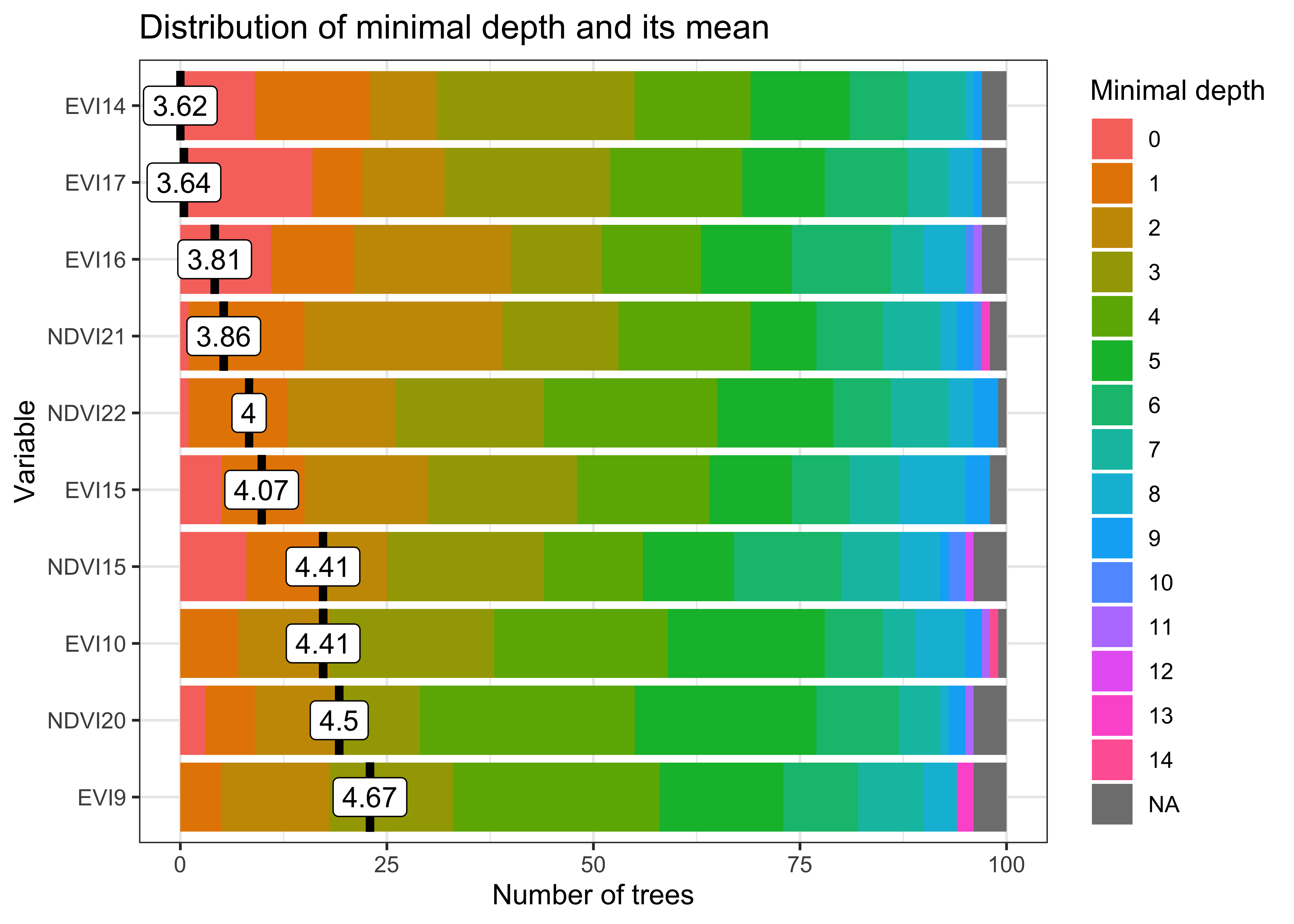

Figure 1.6: Probability map for class Forest.

After completing the classification, we plot the probability maps for class “Forest”. Probability maps are helpful to visualize the degree of confidence the classifier assigns to the labels for each pixel. They can be used to produce uncertainty information and support active learning, as described in Chapter Image classification in data cubes.

Spatial smoothing

When working with big Earth observation data, there is much variability in each class. As a result, some pixels will be misclassified. These errors are more likely to occur in transition areas between classes. To address these problems, sits_smooth() takes a probability cube as input and uses the class probabilities of each pixel’s neighborhood to reduce labeling uncertainty. Plotting the smoothed probability map for class “Forest” shows that most outliers have been removed.

# Perform spatial smoothing
sinop_bayes <- sits_smooth(
  cube = sinop_probs,
  multicores = 2,
  memsize = 8,
  output_dir = "./tempdir/chp3"
)

plot(sinop_bayes, labels = "Forest", palette = "BuGn")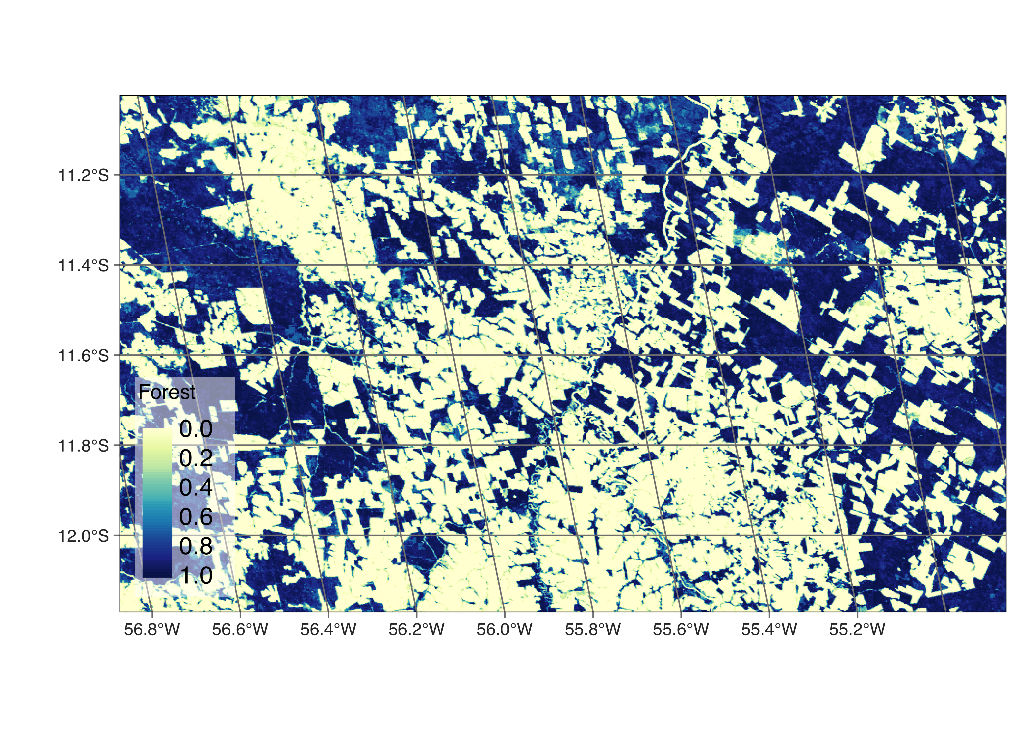

Figure 1.7: Smoothed probability map for class Forest.

Labeling a probability data cube

After removing outliers using local smoothing, the final classification map can be obtained using sits_label_classification(). This function assigns each pixel to the class with the highest probability.

# Label the probability file
sinop_map <- sits_label_classification(
  cube = sinop_bayes,
  output_dir = "./tempdir/chp3"
)

plot(sinop_map, title = "Sinop Classification Map")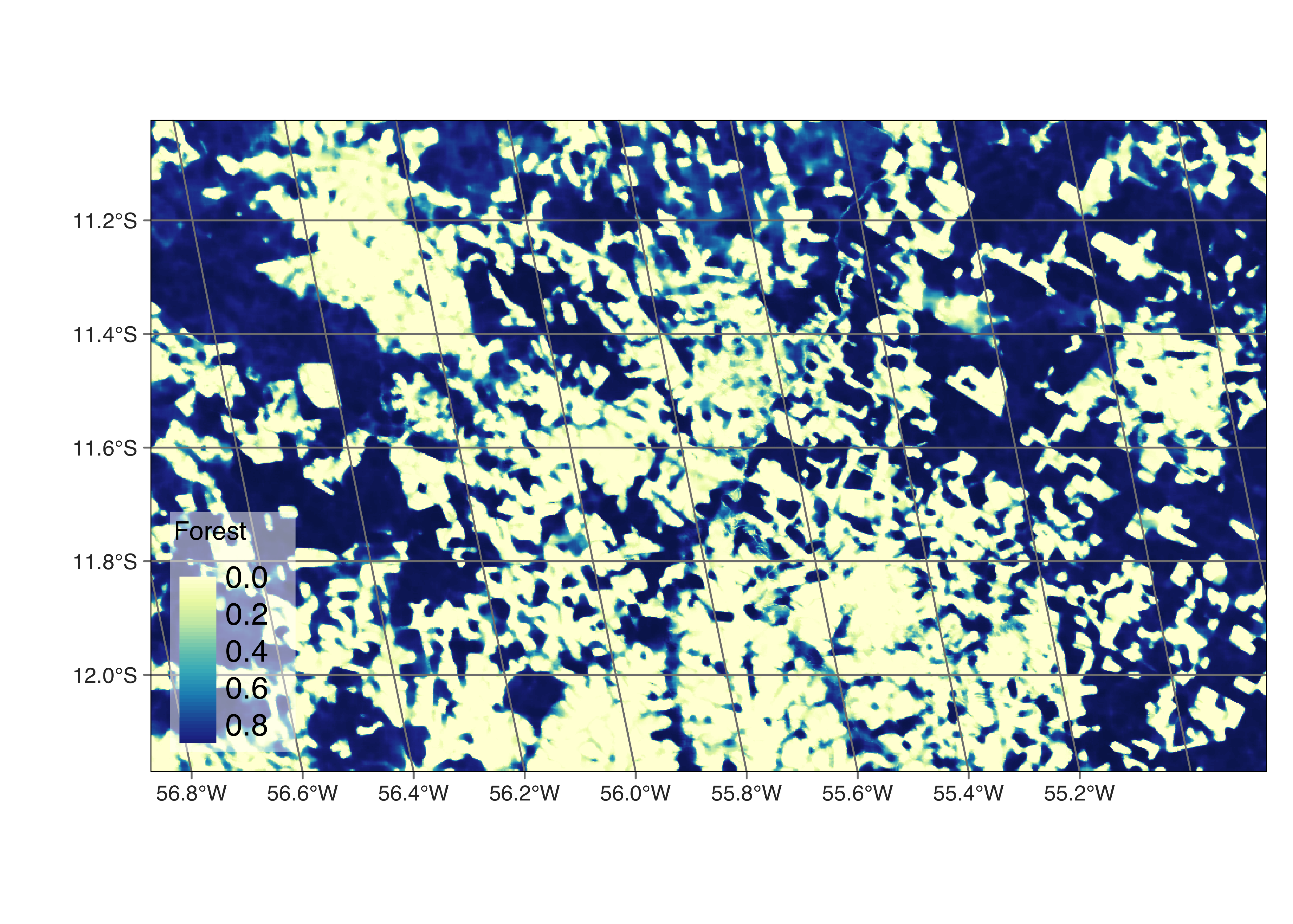

Figure 1.8: Classification map for Sinop.

The resulting classification files can be read by QGIS. Links to the associated files are available in the sinop_map object in the nested table file_info.

# Show the location of the classification file
sinop_map$file_info[[1]]

#> # A tibble: 1 × 12
#>   band  start_date end_date   ncols nrows  xres  yres      xmin      xmax      ymin      ymax path     
#>   <chr> <date>     <date>     <dbl> <dbl> <dbl> <dbl>     <dbl>     <dbl>     <dbl>     <dbl> <chr>    
#> 1 class 2013-09-14 2014-08-29   944   551  232.  232. -6181982. -5963298. -1353336. -1225694. ./tempdi…

As shown in this Introduction, sits provides an end-to-end API to land classification. In what follows, each Chapter provides a detailed description of the training, modeling, and classification workflow.

Acknowledgements

Earth observation data cubes

1 Introduction to sits