8 Computing NDVI and other spectral indices
Configurations to run this chapter
# load "pysits" library
from pysits import *
from pathlib import Path
# set tempdir if it does not exist
tempdir_py = Path.home() / "sitsbook/tempdir/Python/dc_cubeoperations"
tempdir_py.mkdir(parents=True, exist_ok=True)
8.1 Pixel-based and neighborhood-based operations
Pixel-based operations in remote sensing images refer to image processing techniques that operate on individual pixels or cells in an image without considering their spatial relationships with neighboring pixels. These operations are typically applied to each pixel in the image independently; they are used to extract information on spectral, radiometric, or spatial properties. Pixel-based operations produce spectral indexes which combine data from multiple bands.
Neighborhood-based operations are applied to groups of pixels in an image. The neighborhood is typically defined as a rectangular or circular region centered on a given pixel. These operations can be used for removing noise, detecting edges, and sharpening, among other uses.
The sits_apply() function computes new indices from a desired mathematical operation as a function of the bands available on the cube using any valid R expression. It applies the operation for all tiles and all temporal intervals. There are two types of operations in sits_apply():
Pixel-based operations that produce an index based on individual pixels of existing bands. The input bands and indexes should be part of the input data cube and have the same names used in the cube. The new index will be computed for every pixel of all images in the time series. Besides arithmetic operators, the function also accepts vectorized R functions that can be applied to matrices (e.g.,
sqrt(),log(), andsin()).Neighborhood-based operations that produce a derived value based on a window centered around each individual pixel. The available functions are
w_median(),w_sum(),w_mean(),w_min(),w_max(),w_sd()(standard deviation), andw_var()(variance). Users set the window size (only odd values are allowed).
The following examples show how to use sits_apply().
8.2 Computing vegetation indexes
Using vegetation indexes is an established practice in remote sensing. These indexes aim to improve the discrimination of vegetation structure by combining two wavebands, one where leaf pigments reflect incoming light with another where leaves absorb incoming radiation. Green leaves from natural vegetation such as forests have a strong emissivity rate in the near-infrared bands and low emissivity rates in the red bands of the electromagnetic spectrum. These spectral properties are used to calculate the Normalized Difference Vegetation Index (NDVI), a widely used index that is computed as the normalized difference between the values of infra-red and red bands. Including red-edge bands in Sentinel-2 images has broadened the scope of the bands used to calculate these indices [1], [2]. In what follows, we show examples of vegetation index calculation using a Sentinel-2 data cube.
First, we define a data cube for a tile in the state of Rondonia, Brazil, including bands used to compute different vegetation indexes. We regularize the cube using a target resolution of 60-meters to reduce processing time.
# Create an non-regular data cube from AWS
s2_cube <- sits_cube(
    source = "AWS",
    collection = "SENTINEL-S2-L2A-COGS",
    tiles = "20LKP",
    bands = c("B02", "B03", "B04",
              "B05", "B06", "B07",
              "B08", "B8A", "B11",
              "B12","CLOUD"),
    start_date = as.Date("2018-07-01"),
    end_date = as.Date("2018-08-31"))

# Regularize the cube to 15 day intervals
reg_cube <- sits_regularize(
          cube       = s2_cube,
          output_dir = tempdir_r,
          res        = 60,
          period     = "P15D",
          multicores = 4)
# Create an non-regular data cube from AWS
s2_cube = sits_cube(
source = "AWS",
collection = "SENTINEL-S2-L2A-COGS",
tiles = "20LKP",
bands = ("B02", "B03", "B04",
"B05", "B06", "B07",
"B08", "B8A", "B11",
"B12","CLOUD"),
start_date = "2018-07-01",
end_date = "2018-08-31")
# Regularize the cube to 15 day intervals
reg_cube = sits_regularize(
cube = s2_cube,
output_dir = tempdir_py,
res = 60,
period = "P15D",
multicores = 4)There are many options for calculating vegetation indexes using Sentinel-2 bands. The most widely used method combines band B08 (785-899 nm) and band B04 (650-680 nm). Recent works in the literature propose using the red-edge bands B05 (698-713 nm), B06 (733-748 nm), and B07 (773-793 nm) for capturing subtle variations in chlorophyll absorption producing indexes, which are called Normalized Difference Vegetation Red-edge indexes (NDRE) [1]. In a recent review, Chaves et al. argue that red-edge bands are important for distinguishing leaf structure and chlorophyll content of different vegetation species [3]. In the example below, we show how to include indexes in the regular data cube with the Sentinel-2 spectral bands.
We first calculate the NDVI in the usual way, using bands B08 and B04.
# Calculate NDVI index using bands B08 and B04
reg_cube <- sits_apply(reg_cube,
    NDVI = (B08 - B04)/(B08 + B04),
    output_dir = tempdir_r
)

# Plot
plot(reg_cube, band = "NDVI", palette = "RdYlGn")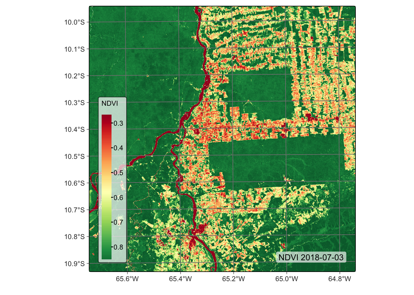
# Calculate NDVI index using bands B08 and B04
reg_cube = sits_apply(reg_cube,
    NDVI = "(B08 - B04)/(B08 + B04)",
    output_dir = tempdir_py
)

# Plot
plot(reg_cube, band = "NDVI", palette = "RdYlGn")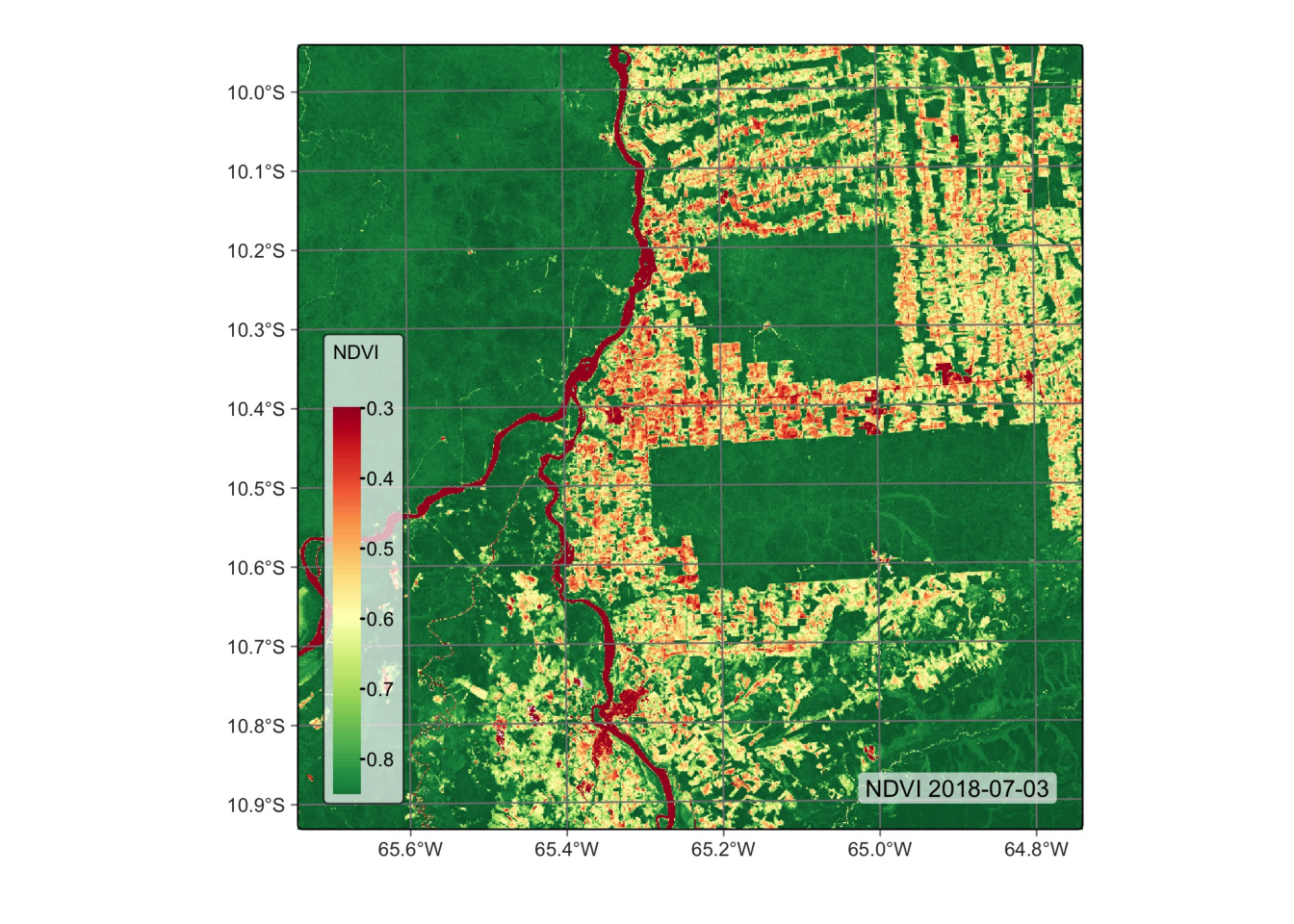
We now compare the traditional NDVI with other vegetation index computed using red-edge bands. The example below such the NDRE1 index, obtained using bands B06 and B05. Sun et al. argue that a vegetation index built using bands B06 and B07 provides a better approximation to leaf area index estimates than NDVI [2]. Notice that the contrast between forests and deforested areas is more robust in the NDRE1 index than with NDVI.
# Calculate NDRE1 index using bands B06 and B05
reg_cube <- sits_apply(reg_cube,
    NDRE1 = (B06 - B05)/(B06 + B05),
    output_dir = tempdir_r
)

# Plot NDRE1 index
plot(reg_cube, band = "NDRE1",  palette = "RdYlGn")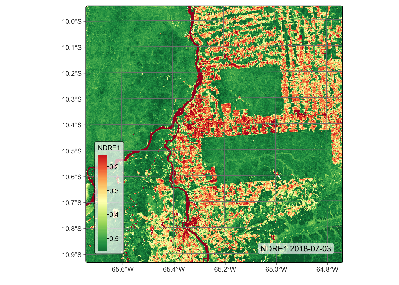
# Calculate NDRE1 index using bands B06 and B05
reg_cube = sits_apply(reg_cube,
    NDRE1 = "(B06 - B05)/(B06 + B05)",
    output_dir = tempdir_py
)

# Plot NDRE1 index
plot(reg_cube, band = "NDRE1",  palette = "RdYlGn")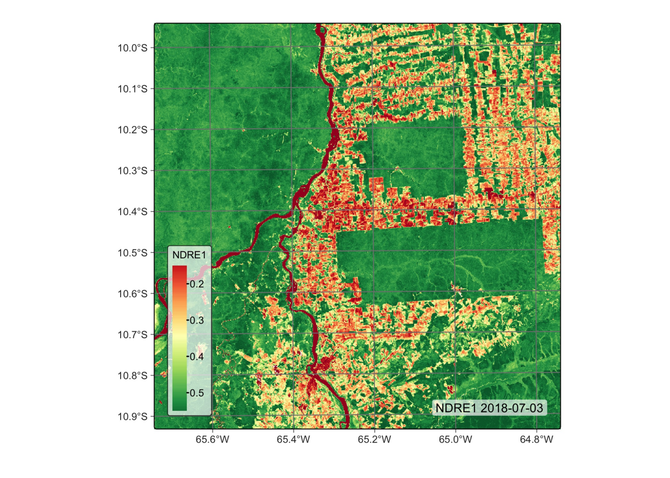
8.3 Spectral indexes for identifying burned areas
Band combinations can also generate spectral indices for detecting degradation by fires, which are an important element in environmental degradation. Forest fires significantly impact emissions and impoverish natural ecosystems [4]. Fires open the canopy, making the microclimate drier and increasing the amount of dry fuel [5]. One well-established technique for detecting burned areas with remote sensing images is the normalized burn ratio (NBR), the difference between the near-infrared and the short wave infrared band, calculated using bands B8A and B12.
# Calculate the NBR index
reg_cube <- sits_apply(reg_cube,
    NBR = (B12 - B8A)/(B12 + B8A),
    output_dir = tempdir_r
)

# Plot the NBR for the first date
plot(reg_cube, band = "NBR", palette = "Reds")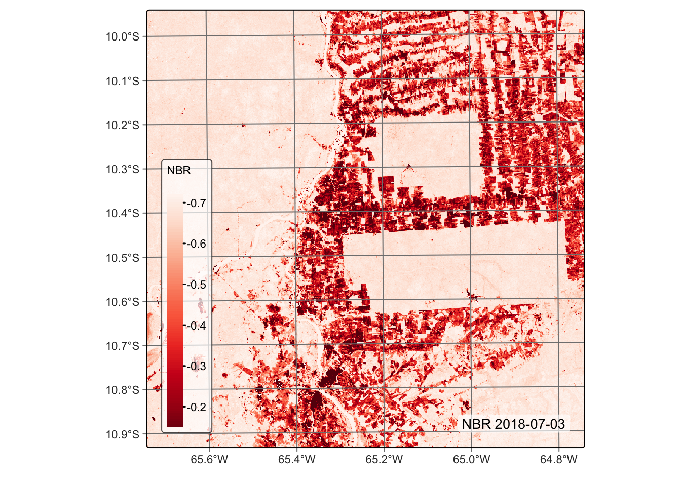
# Calculate the NBR index
reg_cube = sits_apply(reg_cube,
    NBR = "(B12 - B8A)/(B12 + B8A)",
    output_dir = tempdir_py
)

# Plot the NBR for the first date
plot(reg_cube, band = "NBR", palette = "Reds")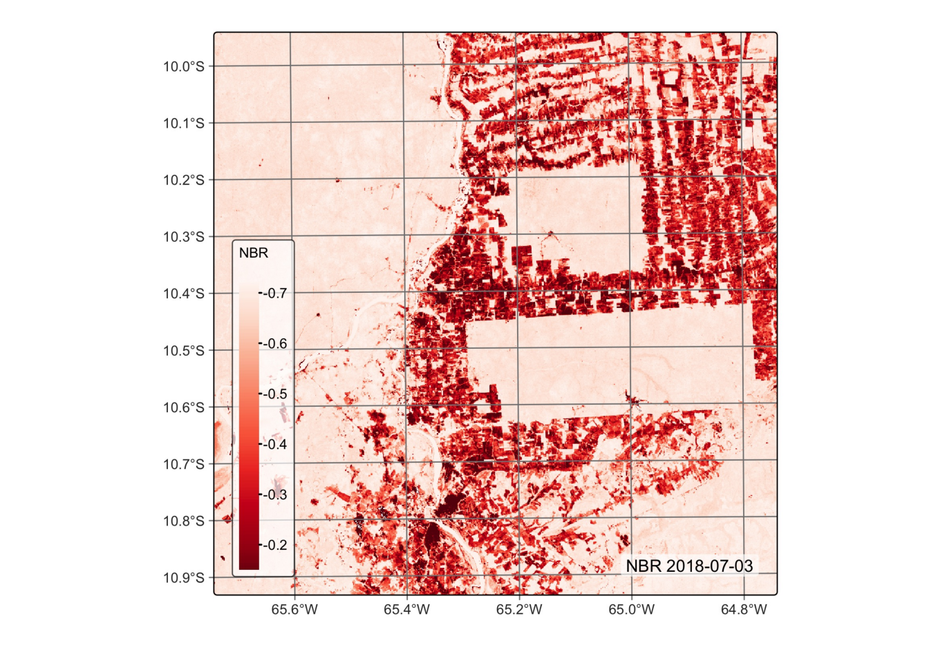
Support for non-normalized indexes
All data cube operations discussed so far produce normalized indexes. By default, the indexes generated by the sits_apply() function are normalized between -1 and 1, scaled by a factor of 0.0001. Normalized indexes are saved as INT2S (Integer with sign). If the normalized parameter is FALSE, no scaling factor will be applied and the index will be saved as FLT4S (Float with sign). The code below shows an example of the non-normalized index, CVI - chlorophyll vegetation index. CVI is a spectral index used to estimate the chlorophyll content and overall health of vegetation. It combines bands in visible and near-infrared (NIR) regions to assess vegetation characteristics. Since CVI is not normalized, we have to set the parameter normalized to FALSE to inform sits_apply() to generate an FLT4S image.
# Calculate the NBR index
reg_cube <- sits_apply(reg_cube,
    CVI = (B8A / B03) * (B05 / B03 ),
    normalized = FALSE,
    output_dir = tempdir_r
)

# Plot
plot(reg_cube, band = "CVI", palette = "Greens")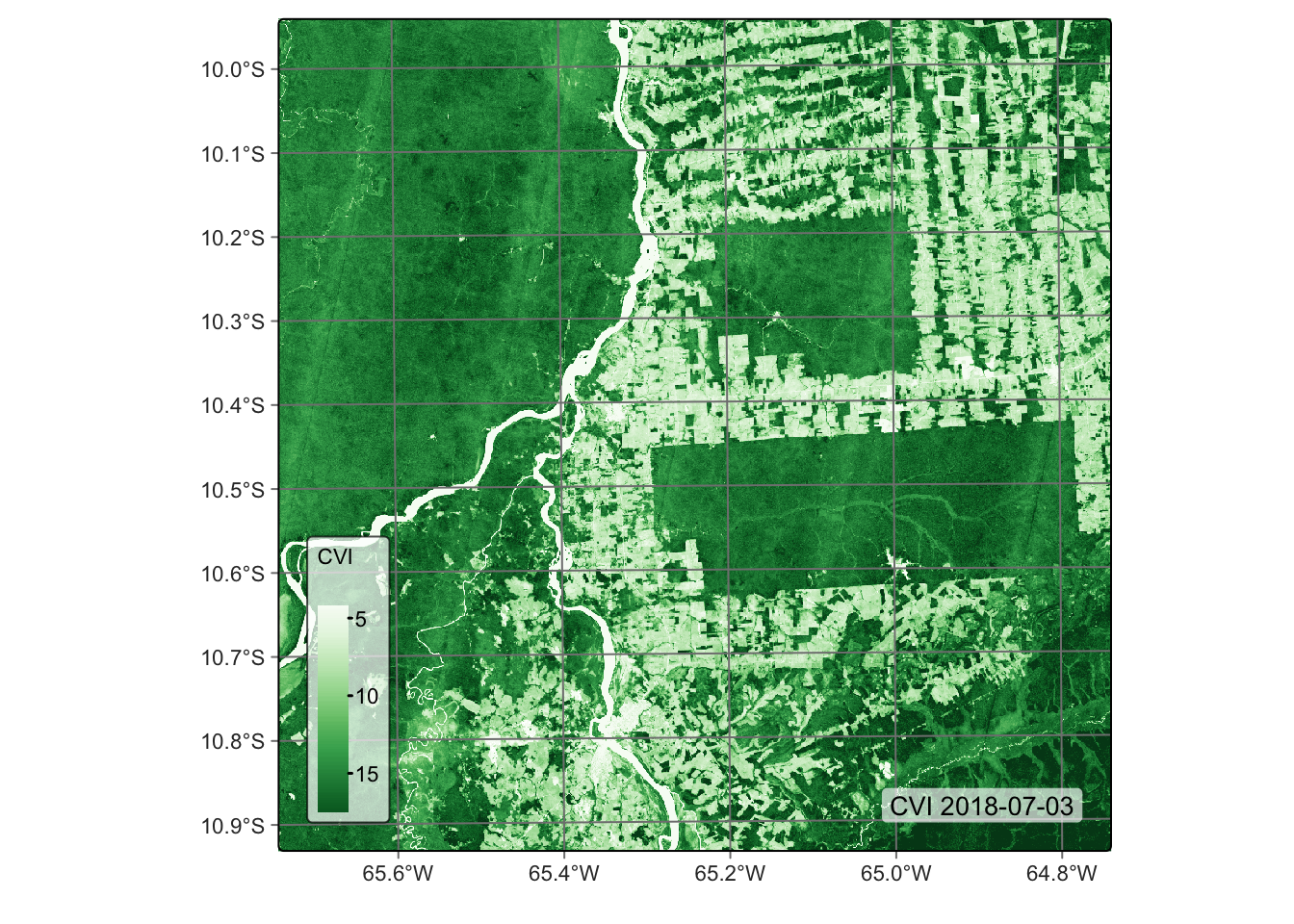
# Calculate the NBR index
reg_cube = sits_apply(reg_cube,
    CVI = "(B8A / B03) * (B05 / B03 )",
    normalized = False,
    output_dir = tempdir_py
)

# Plot
plot(reg_cube, band = "CVI", palette = "Greens")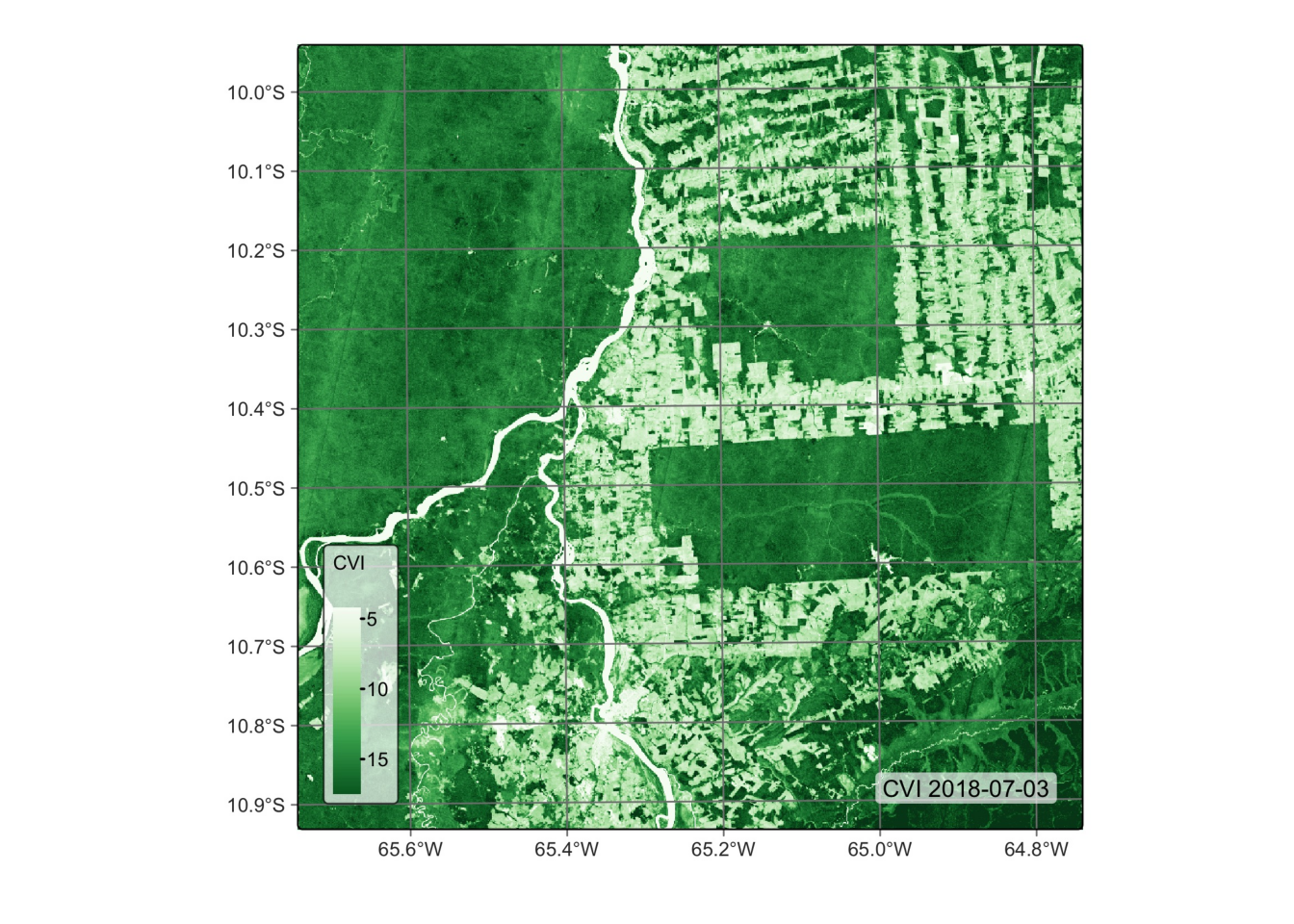
8.4 Summary
In this chapter, we learned how to operate on data cubes, including how to compute spectral indexes, estimate mixture models, and do reducing operations. This chapter concludes our overview of how data cubes work in sits. In the next part, we will describe how to work with time series.