10 Temporal reduction operations
Configurations to run this chapter
# load "pysits" library
from pysits import *
from pathlib import Path
# set tempdir if it does not exist
tempdir_py = Path.home() / "sitsbook/tempdir/Python/dc_reduce"
tempdir_py.mkdir(parents=True, exist_ok=True)
10.1 Introduction
There are cases when users want to combine the values of a time series associated to each pixel of a data cube using reduction operators. In time series analysis, a reduction operator is a function that combines a sequence of data points into a single value. This process involves summarizing or aggregating the information from the time series in a meaningful way. Reduction operators are often used to extract key statistics or features from the data, making it easier to analyze and interpret.
10.2 Methods
To produce temporal combinations, sits provides sits_reduce, with associated functions:
-
t_max(): maximum value of the series. -
t_min(): minimum value of the series -
t_mean(): mean of the series. -
t_median(): median of the series. -
t_std(): standard deviation of the series. -
t_skewness(): skewness of the series. -
t_kurtosis(): kurtosis of the series. -
t_amplitude(): difference between maximum and minimum values of the cycle. A small amplitude means a stable cycle. -
t_fslope(): maximum value of the first slope of the cycle. Indicates when the cycle presents an abrupt change in the curve. The slope between two values relates the speed of the growth or senescence phases -
t_mse(): average spectral energy density. The energy of the time series is distributed by frequency. -
t_fqr(): value of the first quartile of the series (0.25). -
t_tqr(): value of the third quartile of the series (0.75). -
t_iqr(): interquartile range (difference between the third and first quartiles).
The functions t_std(), t_skewness(), t_kurtosis(), and t_mse() produce values greater than the limit of a two-byte integer. Therefore, we save the images generated by them in floating point format.
10.3 Example
The following example shows how to execute a temporal reduction operation.
# Define a region of interest to be enclosed in the data cube
roi <- c(
    "lon_min" = -55.80259,
    "lon_max" = -55.199,
    "lat_min" = -11.80208,
    "lat_max" = -11.49583
)

# Define a data cube in the MPC repository using NDVI MODIS data
ndvi_cube <- sits_cube(
    source = "MPC",
    collection  = "MOD13Q1-6.1",
    bands = c("NDVI"),
    roi = roi,
    start_date =  "2018-05-01",
    end_date = "2018-09-30"
)

# Copy the cube to a local file system
ndvi_cube_local <- sits_cube_copy(
    cube = ndvi_cube,
    output_dir = tempdir_r,
    multicores = 4
)
# Define a region of interest to be enclosed in the data cube
roi = dict(
lon_min = -55.80259,
lon_max = -55.199,
lat_min = -11.80208,
lat_max = -11.49583
)
# Define a data cube in the MPC repository using NDVI MODIS data
ndvi_cube = sits_cube(
source = "MPC",
collection = "MOD13Q1-6.1",
bands = "NDVI",
roi = roi,
start_date = "2018-05-01",
end_date = "2018-09-30"
)
# Copy the cube to a local file system
ndvi_cube_local = sits_cube_copy(
cube = ndvi_cube,
output_dir = tempdir_py,
multicores = 4
)After creating a local data cube based on the contents of the MPC MODIS cube with the NDVI band, we can now compute the maximum NDVI values for each pixel for the images during the period from 2018-05-01 to 2018-09-30.
# create a local directory to store the result of the operation
tempdir_r_ndvi_max <- file.path(tempdir_r, "ndvi_max")
dir.create(tempdir_r_ndvi_max, showWarnings = FALSE)

# Calculate the NBR index
max_ndvi_cube <- sits_reduce(ndvi_cube_local,
    NDVIMAX = t_max(NDVI),
    output_dir = tempdir_r_ndvi_max,
    multicores = 4,
    progress = TRUE
)
plot(max_ndvi_cube, band = "NDVIMAX")
# create a local directory to store the result of the operation
tempdir_py_ndvi_max = tempdir_py / "ndvi_max"
tempdir_py_ndvi_max.mkdir(parents=True, exist_ok=True)
# Calculate the NBR index
max_ndvi_cube = sits_reduce(ndvi_cube_local,
NDVIMAX = "t_max(NDVI)",
output_dir = tempdir_py_ndvi_max,
multicores = 4,
progress = True
)
plot(max_ndvi_cube, band = "NDVIMAX")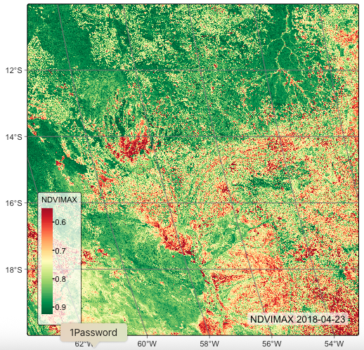
10.4 Summary
Temporal reducing operations in Earth Observation (EO) data cubes are aggregations or summaries performed along the time dimension. These operations compress temporal information—typically multiple observations of the same location over time—into a single value or summary per pixel or area. They are useful for generating cloud-free composites, trend analyses, and preparing data for classification or modeling.