1 A quick tour of SITS

Configurations to run this chapter
# load "pysits" library
from pysits import *
from pathlib import Path
# set tempdir if it does not exist
tempdir_py = Path.home() / "sitsbook/tempdir/Python/intro_quicktour"
tempdir_py.mkdir(parents=True, exist_ok=True)
1.1 Overview
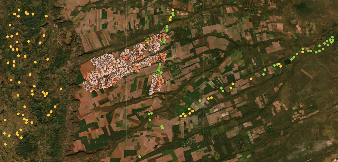
In this chapter, we present a simple example of using sits for agricultural classification. We start by taking a set of samples with land use and land cover types for an area in the Cerrado biome in Brazil, near the city of Luis Eduardo Magalhães in the state of Bahia. These samples were collected by a team of INPE researchers [1].
1.2 Training samples
In this example, we take the data set for agriculture in the municipality of Luis Eduardo Magalhaes (henceforth LEM) as our starting point. This is a common situation in land classification. To be able to obtain time series information, sits requires that the training samples provide, for each sample, information on location, temporal range, and associated label. In this example, we use a data frame with five columns: longitude, latitude, start_date, end_date and label. The training samples are available in the R sitsdata package. Alternative ways of defining data samples include CSV files and shapefiles. Please refer to chapter “Working with time series”.
# Load the samples for LEM from the "sitsdata" package
# select the directory for the samples
samples_dir <- system.file("data", package = "sitsdata")

# retrieve a data.frame with the samples
df_samples_cerrado_lem <- readRDS(file.path(samples_dir, "df_samples_cerrado_lem.rds"))
df_samples_cerrado_lem
# A tibble: 2,302 × 5
longitude latitude start_date end_date label
<dbl> <dbl> <date> <date> <chr>
1 -46.5 -12.3 2019-09-30 2020-09-29 Pasture
2 -46.5 -12.3 2019-09-30 2020-09-29 Pasture
3 -46.4 -12.3 2019-09-30 2020-09-29 Pasture
4 -46.5 -12.3 2019-09-30 2020-09-29 Pasture
5 -46.5 -12.3 2019-09-30 2020-09-29 Pasture
6 -46.5 -12.3 2019-09-30 2020-09-29 Pasture
7 -46.6 -12.4 2019-09-30 2020-09-29 Pasture
8 -46.6 -12.3 2019-09-30 2020-09-29 Pasture
9 -46.5 -12.3 2019-09-30 2020-09-29 Pasture
10 -46.6 -12.4 2019-09-30 2020-09-29 Pasture
# ℹ 2,292 more rows# Load the samples for Mato Grosso from the "sitsdata" package
# select the directory for the samples
samples_file = r_package_dir("data/df_samples_cerrado_lem.rds", package = "sitsdata")
# retrieve a data.frame with the samples
df_samples_cerrado_lem = read_rds(samples_file)
df_samples_cerrado_lem longitude latitude start_date end_date label
0 -46.536000 -12.306000 2019-09-30 2020-09-29 Pasture
1 -46.545000 -12.310000 2019-09-30 2020-09-29 Pasture
2 -46.420000 -12.338000 2019-09-30 2020-09-29 Pasture
3 -46.513000 -12.322000 2019-09-30 2020-09-29 Pasture
4 -46.506000 -12.328000 2019-09-30 2020-09-29 Pasture
... ... ... ... ... ...
2297 -45.871588 -12.401668 2019-09-30 2020-09-29 Cerrado
2298 -45.871573 -12.426070 2019-09-30 2020-09-29 Cropland_2_cycles
2299 -45.869899 -12.429560 2019-09-30 2020-09-29 Cropland_2_cycles
2300 -45.869663 -12.430767 2019-09-30 2020-09-29 Cropland_2_cycles
2301 -45.868158 -12.430211 2019-09-30 2020-09-29 Cropland_2_cycles
[2302 rows x 5 columns]The data set contains 2,302 samples divided into four classes: (a) “Cerrado,” which corresponds to the natural vegetation associated with the Brazilian savanna; (b) “Cropland_1_cycle,” temporary agriculture (mostly soybeans) planted in a single cycle from October to March; (c) “Cropland_2_cycles,” temporary agriculture planted in two cycles, the first from October to March and the second from April to July; (d) “Pasture,” areas for cattle raising. For convenience, we present a high-resolution image of the area with the location of the samples.
1.3 Creating a data cube based on the ground truth samples
There are two kinds of data cubes in sits: (a) non-regular data cubes generated by selecting ARD image collections on cloud providers such as AWS and Planetary Computer; (b) regular data cubes with images fully covering a chosen area, where each image has the same spectral bands and spatial resolution, and images follow a set of adjacent and regular time intervals. Machine learning applications need regular data cubes. Please refer to Chapter Building regular data cubes for further details.
The first steps in using sits are: (a) select an analysis-ready data image collection available from a cloud provider or stored locally using sits_cube(); (b) if the collection is not regular, use sits_regularize() to build a regular data cube.
This example builds a data cube from local images already organized as a regular data cube available in the Brazil Data Cube (“BDC”). The data cube is composed of CBERS-4 and CBERS-4A images for the LEM data set, covering the training samples. The images are taken with the WFI (wide field imager) sensor with 64-meter resolution. All images have indices NDVI and EVI covering a one-year period from 2019-09-30 to 2020-09-29 (we use “year-month-day” for dates). There are 24 time instances, each covering a 16-day period. We first define the region of interest using the bounding box of the LEM data set, and then define a data cube in the BDC repository based on this region. This data cube will be composed of the CBERS images that intersect with the region of interest.
# Find the the bounding box of the data
lat_max <- max(df_samples_cerrado_lem[["latitude"]])
lat_min <- min(df_samples_cerrado_lem[["latitude"]])
lon_max <- max(df_samples_cerrado_lem[["longitude"]])
lon_min <- min(df_samples_cerrado_lem[["longitude"]])

# Define the roi for the LEM dataset
roi_lem <- c(
    "lat_max" = lat_max,
    "lat_min" = lat_min,
    "lon_max" = lon_max,
    "lon_min" = lon_min)

# Define a data cube in the BDC repository based on the LEM ROI
bdc_cube <- sits_cube(
    source = "BDC",
    collection  = "CBERS-WFI-16D",
    bands = c("NDVI", "EVI"),
    roi = roi_lem,
    start_date = "2019-09-30",
    end_date = "2020-09-29"
)
# Find the the bounding box of the data
lat_max = max(df_samples_cerrado_lem["latitude"])
lat_min = min(df_samples_cerrado_lem["latitude"])
lon_max = max(df_samples_cerrado_lem["longitude"])
lon_min = min(df_samples_cerrado_lem["longitude"])
# Define the roi for the LEM dataset
roi_lem = dict(
lat_max = lat_max,
lat_min = lat_min,
lon_max = lon_max,
lon_min = lon_min
)
# Define a data cube in the BDC repository based on the LEM ROI
bdc_cube = sits_cube(
source = "BDC",
collection = "CBERS-WFI-16D",
bands = ("NDVI", "EVI"),
roi = roi_lem,
start_date = "2019-09-30",
end_date = "2020-09-29"
)The next step is to copy the data cube to a local directory for further processing. When using a region of interest to select a part of an ARD collection, sits intersects the region with the tiles of that collection. Thus, when one wants to get a subset of a tile, it is better to copy this subset to the local computer. After downloading the data, we use plot() to view it. The plot() function, by default, selects the image with the least cloud cover.
# Copy the region of interest to a local directory
lem_cube <- sits_cube_copy(
    cube = bdc_cube,
    roi = roi_lem,
    output_dir = tempdir_r
)

# Plot the cube
plot(lem_cube, palette = "RdYlGn")
# Copy the region of interest to a local directory
lem_cube = sits_cube_copy(
cube = bdc_cube,
roi = roi_lem,
output_dir = tempdir_py
)
# Plot the cube
plot(lem_cube, palette = "RdYlGn")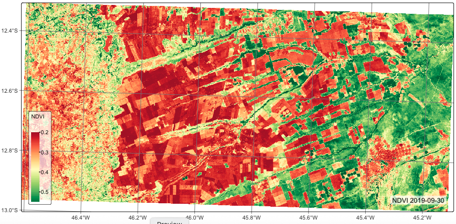
The object returned by sits_cube() and by sits_cube_copy() contains the metadata describing the contents of the data cube. It includes the data source and collection, satellite, sensor, tile in the collection, bounding box, projection, and list of files. Each file refers to one band of an image at one of the temporal instances of the cube. Since data cubes obtained from the BDC are already regularized, there is no need to run sits_regularize(). Please refer to chapter “Building regular EO data cubes” for information on dealing with non-regular ARD collections.
# Show the description of the data cube
lem_cube
# A tibble: 1 × 12
source collection satellite sensor tile xmin xmax ymin ymax crs
<chr> <chr> <chr> <chr> <chr> <dbl> <dbl> <dbl> <dbl> <chr>
1 BDC CBERS-WFI-16D CBERS-4 WFI 007004 5.79e6 5.95e6 9.88e6 9.96e6 "PRO…
# ℹ 2 more variables: labels <list>, file_info <list># Show the description of the data cube
lem_cube source collection satellite sensor ... ymin ymax crs file_info
0 BDC CBERS-WFI-16D CBERS-4 WFI ... 9876544.0 9955136.0 PROJCRS["unknown",\n BASEGEOGCRS["unknown",... fid band da...
[1 rows x 11 columns]The list of image files that make up the data cube is stored as a data frame in the column file_info. For each file, sits stores information about the spectral band, reference date, size, spatial resolution, coordinate reference system, bounding box, path to the file location, and cloud cover information (when available).
# Show information on the images files which are part of a data cube
lem_cube$file_info[[1]]
# A tibble: 48 × 13
fid band date ncols nrows xres yres xmin xmax ymin ymax
<chr> <chr> <date> <dbl> <dbl> <dbl> <dbl> <dbl> <dbl> <dbl> <dbl>
1 CB4-16D… EVI 2019-09-30 2539 1228 64 64 5.79e6 5.95e6 9.88e6 9.96e6
2 CB4-16D… NDVI 2019-09-30 2539 1228 64 64 5.79e6 5.95e6 9.88e6 9.96e6
3 CB4-16D… EVI 2019-10-16 2539 1228 64 64 5.79e6 5.95e6 9.88e6 9.96e6
4 CB4-16D… NDVI 2019-10-16 2539 1228 64 64 5.79e6 5.95e6 9.88e6 9.96e6
5 CB4-16D… EVI 2019-11-01 2539 1228 64 64 5.79e6 5.95e6 9.88e6 9.96e6
6 CB4-16D… NDVI 2019-11-01 2539 1228 64 64 5.79e6 5.95e6 9.88e6 9.96e6
7 CB4-16D… EVI 2019-11-17 2539 1228 64 64 5.79e6 5.95e6 9.88e6 9.96e6
8 CB4-16D… NDVI 2019-11-17 2539 1228 64 64 5.79e6 5.95e6 9.88e6 9.96e6
9 CB4-16D… EVI 2019-12-03 2539 1228 64 64 5.79e6 5.95e6 9.88e6 9.96e6
10 CB4-16D… NDVI 2019-12-03 2539 1228 64 64 5.79e6 5.95e6 9.88e6 9.96e6
# ℹ 38 more rows
# ℹ 2 more variables: crs <chr>, path <chr># Show information on the images files which are part of a data cube
lem_cube["file_info"][0].head(5) fid band date ncols ... ymin ymax crs path
0 CB4-16D_V2_007004_20190930 EVI 2019-09-30 2539.0 ... 9876544.0 9955136.0 PROJCRS["unknown",\n BASEGEOGCRS["unknown",... /Users/gilbertocamara/sitsbook/tempdir/R/intro...
1 CB4-16D_V2_007004_20190930 NDVI 2019-09-30 2539.0 ... 9876544.0 9955136.0 PROJCRS["unknown",\n BASEGEOGCRS["unknown",... /Users/gilbertocamara/sitsbook/tempdir/R/intro...
2 CB4-16D_V2_007004_20191016 EVI 2019-10-16 2539.0 ... 9876544.0 9955136.0 PROJCRS["unknown",\n BASEGEOGCRS["unknown",... /Users/gilbertocamara/sitsbook/tempdir/R/intro...
3 CB4-16D_V2_007004_20191016 NDVI 2019-10-16 2539.0 ... 9876544.0 9955136.0 PROJCRS["unknown",\n BASEGEOGCRS["unknown",... /Users/gilbertocamara/sitsbook/tempdir/R/intro...
4 CB4-16D_V2_007004_20191101 EVI 2019-11-01 2539.0 ... 9876544.0 9955136.0 PROJCRS["unknown",\n BASEGEOGCRS["unknown",... /Users/gilbertocamara/sitsbook/tempdir/R/intro...
[5 rows x 13 columns]A key attribute of a data cube is its timeline, as shown below. The command sits_timeline() lists the temporal references associated to sits objects, including samples, data cubes and models.
# Show the R object that describes the data cube
sits_timeline(lem_cube)
[1] "2019-09-30" "2019-10-16" "2019-11-01" "2019-11-17" "2019-12-03"
[6] "2019-12-19" "2020-01-01" "2020-01-17" "2020-02-02" "2020-02-18"
[11] "2020-03-05" "2020-03-21" "2020-04-06" "2020-04-22" "2020-05-08"
[16] "2020-05-24" "2020-06-09" "2020-06-25" "2020-07-11" "2020-07-27"
[21] "2020-08-12" "2020-08-28" "2020-09-13" "2020-09-29"# Show the R object that describes the data cube
sits_timeline(lem_cube)['2019-09-30', '2019-10-16', '2019-11-01', '2019-11-17', '2019-12-03', '2019-12-19', '2020-01-01', '2020-01-17', '2020-02-02', '2020-02-18', '2020-03-05', '2020-03-21', '2020-04-06', '2020-04-22', '2020-05-08', '2020-05-24', '2020-06-09', '2020-06-25', '2020-07-11', '2020-07-27', '2020-08-12', '2020-08-28', '2020-09-13', '2020-09-29']The timeline of lem_cube has 24 intervals with a temporal difference of 16 days. The chosen dates capture the agricultural calendar in the west of Bahia in Brazil. The agricultural year starts in September-October with the sowing of the summer crop (usually soybeans), which is harvested in February-March. Then the winter crop (mostly Corn, Cotton, or Millet) is planted in March and harvested in June-July. For LULC classification, the training samples and the data cube should share a timeline with the same number of intervals and similar start and end dates.
1.4 The time series tibble
To handle time series information, sits uses a tibble. Tibbles are extensions of the data.frame tabular data structures provided by the tidyverse set of packages. In this chapter, we will use a training set with 1,101 time series obtained from MODIS MOD13Q1 images. Each series has two indexes (NDVI and EVI). To obtain the time series, we need two inputs:
A CSV file, shapefile or a data.frame containing information on the location of the sample and date of validity. The following information is required:
longitude,latitude,start_date,end_date,class. It can either be provided as columns of a data.frame or a CSV file, or as attributes of a shapefile. Please refer to Chapter “Working with time series” for more information.A regular data cube which covers the dates indicated in the sample file. Each sample will be located in the data cube based on its longitude and latitude, and the time series is extracted based on the start and end dates and on the available bands of the cube.
In what follows, we use the data frame with the LEM samples. The data.frame contains spatial and temporal information and the label assigned to the sample. Based on this information, we will retrieve the time series from the BDC cube using sits_get_data(). In general, it is necessary to regularize the data cube so that all time series have the same dates. In our case, we use a regular data cube provided by the BDC repository.
# Retrieve the time series for each samples based on a data.frame
samples_lem_time_series <- sits_get_data(
    cube = lem_cube,
    samples = df_samples_cerrado_lem
)
# Retrieve the time series for each samples based on a data.frame
samples_lem_time_series = sits_get_data(
cube = lem_cube,
samples = df_samples_cerrado_lem
)The time series tibble contains data and metadata. The first six columns contain the metadata: spatial and temporal information, the label assigned to the sample, and the data cube from where the data has been extracted. The time_series column contains the time series data for each spatiotemporal location. This data is also organized as a tibble, with a column with the dates and the other columns with the values for each spectral band. The time series can be displayed by showing the time_series nested column.
# Load the time series for the first MODIS sample for Mato Grosso
samples_lem_time_series[1,]$time_series[[1]]
# A tibble: 24 × 3
Index EVI NDVI
<date> <dbl> <dbl>
1 2019-09-30 0.203 0.240
2 2019-10-16 0.254 0.352
3 2019-11-01 0.297 0.390
4 2019-11-17 0.344 0.542
5 2019-12-03 0.174 0.206
6 2019-12-19 0.353 0.498
7 2020-01-01 0.433 0.659
8 2020-01-17 0.441 0.595
9 2020-02-02 0.431 0.674
10 2020-02-18 0.565 0.672
# ℹ 14 more rows# Load the time series for the first MODIS sample for Mato Grosso
samples_lem_time_series["time_series"][0] Index EVI NDVI
0 2019-09-30 0.2031 0.2403
1 2019-10-16 0.2537 0.3517
2 2019-11-01 0.2973 0.3899
3 2019-11-17 0.3443 0.5415
4 2019-12-03 0.1740 0.2059
.. ... ... ...
19 2020-07-27 0.2504 0.3612
20 2020-08-12 0.2272 0.3378
21 2020-08-28 0.2080 0.2962
22 2020-09-13 0.2077 0.2755
23 2020-09-29 0.2018 0.2866
[24 rows x 3 columns]The distribution of samples per class can be obtained using the summary() command. The classification schema uses four labels, two associated with crops (Cropland_2_cycles, Cropland_1_cycle), one with natural vegetation (Cerrado), and one with Pasture.
# Show the summary of the time series sample data
summary(samples_lem_time_series)
# A tibble: 4 × 3
label count prop
<chr> <int> <dbl>
1 Cerrado 136 0.0592
2 Cropland_1_cycle 1250 0.544
3 Cropland_2_cycles 790 0.344
4 Pasture 123 0.0535# Show the summary of the time series sample data
summary(samples_lem_time_series) label count prop
1 Cerrado 136 0.059156
2 Cropland_1_cycle 1250 0.543715
3 Cropland_2_cycles 790 0.343628
4 Pasture 123 0.053502The sample dataset is highly imbalanced. To improve performance, we will produce a balanced set after obtaining the time series, as seen below. The sits_reduce_imbalance() function will reduce the maximum number of samples per class to 256 and increase the minimum number to 100. This procedure is recommended to improve the performance of the classification model. The parameter n_samples_over selects the minimum number of samples of the less frequent classes, and the parameter n_samples_under indicates the maximum number of samples for the more frequent ones.
# Reduce imbalance between the classes
samples_lem <- sits_reduce_imbalance(
    samples_lem_time_series,
    n_samples_over = 150,
    n_samples_under = 300
)
# Reduce imbalance between the classes
samples_lem = sits_reduce_imbalance(
samples_lem_time_series,
n_samples_over = 150,
n_samples_under = 300
)The new distribution of samples per class can be obtained using the summary() command. It should show a more balanced data set.
# Show the summary of the balanced time series sample data
summary(samples_lem)
# A tibble: 4 × 3
label count prop
<chr> <int> <dbl>
1 Cerrado 150 0.159
2 Cropland_1_cycle 320 0.339
3 Cropland_2_cycles 324 0.343
4 Pasture 150 0.159# Show the summary of the balanced time series sample data
summary(samples_lem) label count prop
1 Cerrado 150 0.158898
2 Cropland_1_cycle 320 0.338983
3 Cropland_2_cycles 324 0.343220
4 Pasture 150 0.158898It is helpful to plot the dispersion of the time series. In what follows, for brevity, we will filter only one label (Cropland_2_cycles) and select one index (NDVI).
# Select all samples with label "Cropland_2_cycles" using `dplyr::filter`
# since the label attribute is a column of the samples data.frame
samples_cropland_2cycles <- dplyr::filter(
    samples_lem,
    label == "Cropland_2_cycles"
)

# Select the NDVI band values using sits_select
# because band values are in a nested data.frame
samples_crops_2cycles_ndvi <- sits_select(
    samples_cropland_2cycles,
    bands = "NDVI"
)

# plot the samples for label Cropland_2_cycles and band NDVI
plot(samples_crops_2cycles_ndvi)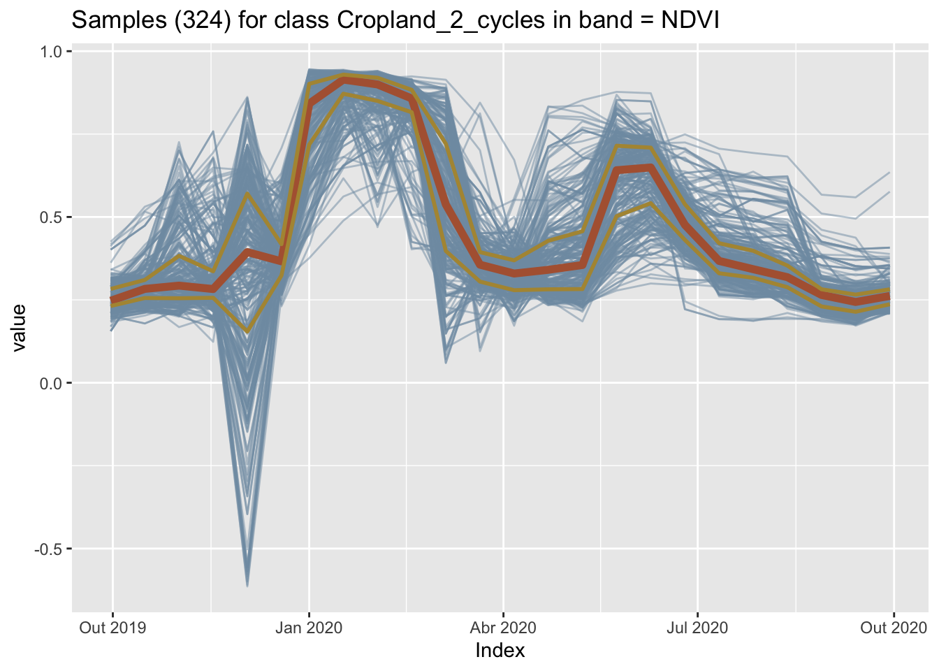
# Select all samples with label "Cropland_2_cycles" using `query`
# since the label attribute is a column of the samples data.frame
samples_crops_2cycles = samples_lem.query('label == "Cropland_2_cycles"')

# Select the NDVI band values using sits_select
# because band values are in a nested data.frame
samples_crops_2cycles_ndvi = sits_select(samples_crops_2cycles, bands = "NDVI")

# plot the samples for label Cropland_2_cycles and band NDVI
plot(samples_crops_2cycles_ndvi)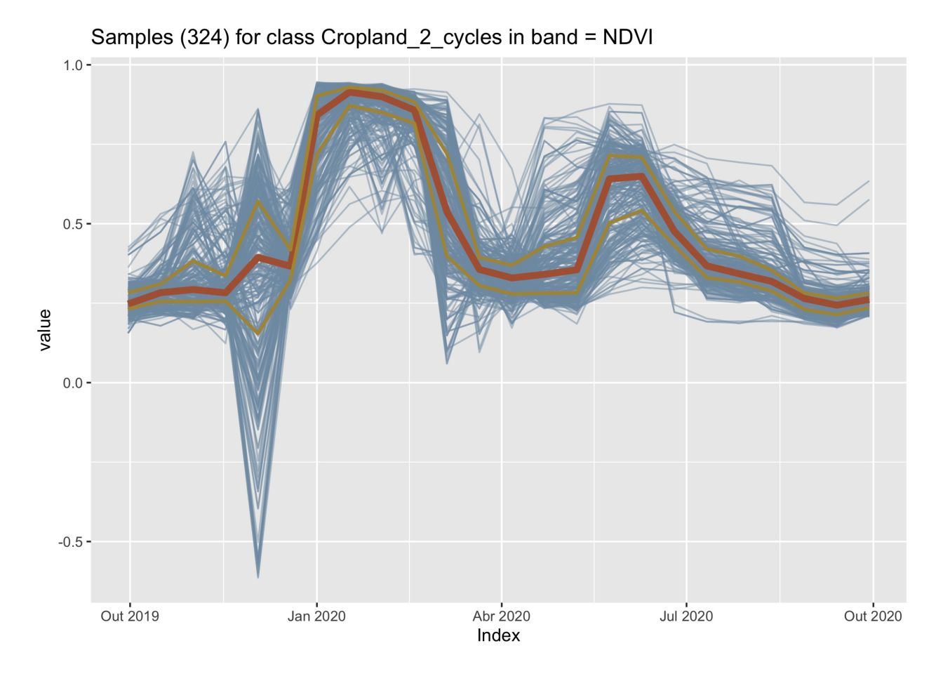
The figure above shows all the time series associated with the label Cropland_2_cycles and the band NDVI (in light blue), highlighting the median (shown in dark red) and the first and third quartiles (shown in brown). The two-crop-cycles pattern is clearly visible. The spikes at the end of the year are due to high cloud cover.
1.5 Training a machine learning model
The next step is to train a machine learning (ML) model using sits_train(). It takes two inputs, samples (a time series tibble) and ml_method (a function that implements a machine learning algorithm). The result is a model that is used for classification. Each ML algorithm requires specific parameters that are user-controllable. For novice users, sits provides default parameters that produce good results. Please see Chapter Machine learning algorithms for image time series for more details.
To build the classification model, we use a Random Forest model called by sits_rfor(). Results from the Random Forest model can vary between different runs, due to the stochastic nature of the algorithm. In the code fragment below, we set the seed of R’s pseudo-random number generator explicitly to ensure results don’t change when running multiple times. This is done for documentation purposes.
set.seed(03022024)

# Train a random forest model
rf_model <- sits_train(
    samples = samples_lem,
    ml_method = sits_rfor()
)

# Plot the most important variables of the model
plot(rf_model)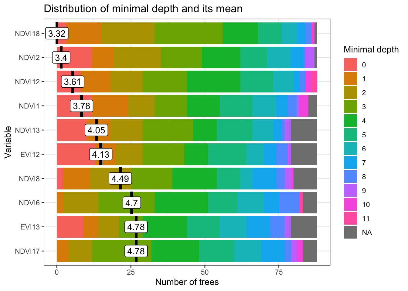
r_set_seed(3022024)

# Train a Random Forest model
rf_model = sits_train(
    samples = samples_lem,
    ml_method = sits_rfor()
)

# Plot the most important variables of the model
plot(rf_model)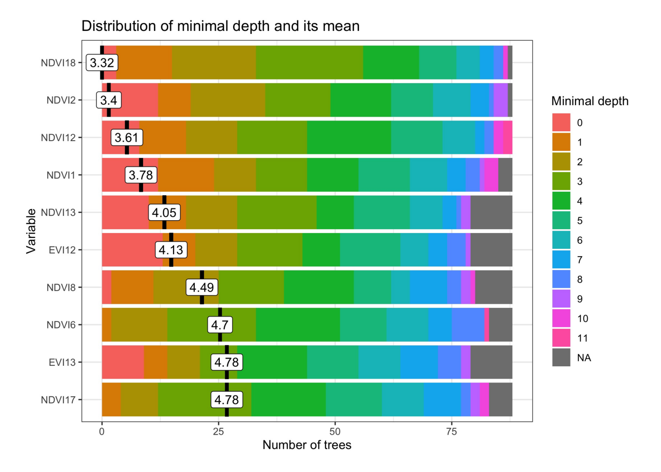
1.6 Data cube classification
After training the machine learning model, the next step is to classify the data cube using sits_classify(). This function produces a set of raster probability maps, one for each class. For each of these maps, the value of a pixel is proportional to the probability that it belongs to the class. This function has two mandatory parameters: data, the data cube or time series tibble to be classified; and ml_model, the trained ML model. Optional parameters include: (a) multicores, number of cores to be used; (b) memsize, RAM used in the classification; (c) output_dir, the directory where the classified raster files will be written. Details of the classification process are available in Chapter Classification of raster data cubes.
# Classify the data cube to produce a map of probabilities
lem_probs <- sits_classify(
    data = lem_cube,
    ml_model = rf_model,
    multicores = 2,
    memsize = 8,
    output_dir = tempdir_r
)

# Plot the probability cube for class Forest
plot(lem_probs, labels = "Cropland_2_cycles", palette = "YlOrBr")
# Classify the data cube to produce a map of probabilities
lem_probs = sits_classify(
data = lem_cube,
ml_model = rf_model,
multicores = 2,
memsize = 8,
output_dir = tempdir_py
)
# Plot the probability cube for class Forest
plot(lem_probs, labels = "Cropland_2_cycles", palette = "YlOrBr")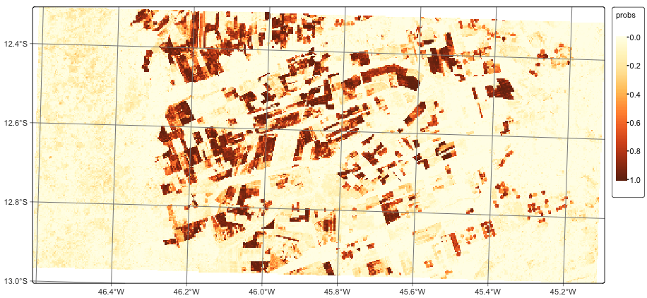
After completing the classification, we plot the probability maps for the class Cropland_2_cycles. Probability maps help visualize the degree of confidence the classifier assigns to the labels for each pixel. They can be used to produce uncertainty information and support active learning, as described in Chapter Uncertainty and active learning.
1.7 Spatial smoothing
When working with big Earth observation data, there is much variability within each class. As a result, some pixels will be misclassified. These errors are more likely to occur in transition areas between classes. To address these problems, sits_smooth() takes a probability cube as input and uses the class probabilities of each pixel’s neighborhood to reduce labeling uncertainty. Plotting the smoothed probability map for the class Forest shows that most outliers have been removed.
# Perform spatial smoothing
lem_smooth <- sits_smooth(
    cube = lem_probs,
    multicores = 2,
    memsize = 8,
    output_dir = tempdir_r
)

plot(lem_smooth, labels = "Cropland_2_cycles", palette = "YlOrBr")
# Perform spatial smoothing
lem_smooth = sits_smooth(
cube = lem_probs,
multicores = 2,
memsize = 8,
output_dir = tempdir_py
)
plot(lem_smooth, labels = "Cropland_2_cycles", palette = "YlOrBr")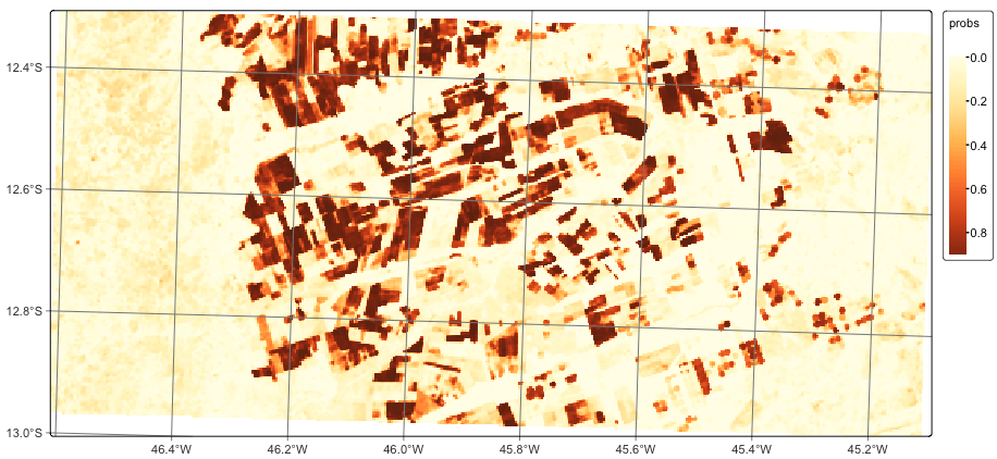
1.8 Labeling a probability data cube
After removing outliers using local smoothing, the final classification map can be obtained using sits_label_classification(). This function assigns each pixel to the class with the highest probability.
# Label the probability file
lem_map <- sits_label_classification(
    cube = lem_smooth,
    output_dir = tempdir_r
)

plot(lem_map)
# Label the probability file
lem_map = sits_label_classification(
cube = lem_smooth,
output_dir = tempdir_py
)
plot(lem_map)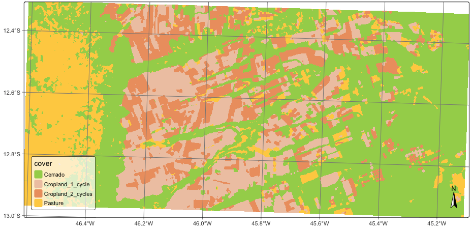
1.9 Summary
This chapter provides an introduction to the main workflow of the sits package, starting from the definition of a data cube from an ARD image collection. Then, we show how to create a regular data cube and how to extract time series using ground truth data. Next, we present a simple way to define machine learning models and how to use them for classifying data cubes. All functions are simple and direct. Once you learn the basic workflow, it becomes easier to understand more detailed examples of sits in the next chapter.