13 Hierarchical clustering of time series
Configurations to run this chapter
# load "pysits" library
from pysits import *
13.1 Introduction
Given a set of training samples, experts should first cross-validate the training set to assess their inherent prediction error. The results show whether the data is internally consistent. Since cross-validation does not predict actual model performance, this chapter provides additional tools for improving the quality of training sets. More detailed information is available in Topic Validation and accuracy measurements.
13.2 Dataset used in this chapter
The examples of this chapter use the cerrado_2classes data, a set of time series for the Cerrado region of Brazil, the second largest biome in South America with an area of more than 2 million \(km^2\). The data contains 746 samples divided into 2 classes (Cerrado and Pasture). Each time series covers 12 months (23 data points) from MOD13Q1 product, and has 2 bands (EVI, and NDVI).
# Show the summary of the cerrado_2_classes dataset
summary(cerrado_2classes)
# A tibble: 2 × 3
label count prop
<chr> <int> <dbl>
1 Cerrado 400 0.536
2 Pasture 346 0.464# Show the summary of the cerrado_2_classes dataset
summary(cerrado_2classes) label count prop
1 Cerrado 400 0.536193
2 Pasture 346 0.46380713.3 Hierarchical clustering for sample quality control
The package provides two clustering methods to assess sample quality: Agglomerative Hierarchical Clustering (AHC) and Self-organizing Maps (SOM). These methods have different computational complexities. AHC has a computational complexity of \(\mathcal{O}(n^2)\), given the number of time series \(n\), whereas SOM complexity is linear. For large data, AHC requires substantial memory and running time; in these cases, SOM is recommended. This section describes how to run AHC in sits. The SOM-based technique is presented in the next section.
AHC computes the dissimilarity between any two elements from a dataset. Depending on the distance functions and linkage criteria, the algorithm decides which two clusters are merged at each iteration. This approach is helpful for exploring samples due to its visualization power and ease of use [1]. In sits, AHC is implemented using sits_cluster_dendro().
# Take a set of patterns for 2 classes
# Create a dendrogram, plot, and get the optimal cluster based on ARI index
clusters <- sits_cluster_dendro(
    samples = cerrado_2classes,
    bands = c("NDVI", "EVI"),
    dist_method = "dtw_basic",
    linkage =  "ward.D2")
# Take a set of patterns for 2 classes
# Create a dendrogram, plot, and get the optimal cluster based on ARI index
clusters = sits_cluster_dendro(
    samples = cerrado_2classes,
    bands = ("NDVI", "EVI"),
    dist_method = "dtw_basic",
    linkage =  "ward.D2")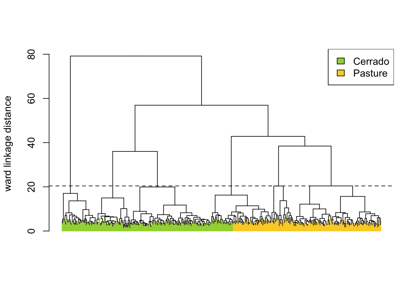
The sits_cluster_dendro() function has one mandatory parameter (samples), with the samples to be evaluated. Optional parameters include bands, dist_method, and linkage. The dist_method parameter specifies how to calculate the distance between two time series. We recommend a metric that uses dynamic time warping (DTW) [2], as DTW is a reliable method for measuring differences between satellite image time series [3]. The options available in sits are based on those provided by package dtwclust, which include dtw_basic, dtw_lb, and dtw2. Please check ?dtwclust::tsclust for more information on DTW distances.
The linkage parameter defines the distance metric between clusters. The recommended linkage criteria are: complete or ward.D2. Complete linkage prioritizes the within-cluster dissimilarities, producing clusters with shorter distance samples, but results are sensitive to outliers. As an alternative, Ward proposes to use the sum-of-squares error to minimize data variance [4]; his method is available as ward.D2 option to the linkage parameter. To cut the dendrogram, the sits_cluster_dendro() function computes the adjusted rand index (ARI) [5], returning the height where the cut of the dendrogram maximizes the index. In the example, the ARI index indicates that there are six clusters. The result of sits_cluster_dendro() is a time series tibble with one additional column called “cluster”. The function sits_cluster_frequency() provides information on the composition of each cluster.
# Show clusters samples frequency
sits_cluster_frequency(clusters)
            1   2   3   4   5   6 Total
  Cerrado 203  13  23  80   1  80   400
  Pasture   2 176  28   0 140   0   346
  Total   205 189  51  80 141  80   746
# Show clusters samples frequency
sits_cluster_frequency(clusters) 1 2 3 4 5 6 Total
Cerrado 203.0 13.0 23.0 80.0 1.0 80.0 400.0
Pasture 2.0 176.0 28.0 0.0 140.0 0.0 346.0
Total 205.0 189.0 51.0 80.0 141.0 80.0 746.0The cluster frequency table shows that each cluster has a predominance of either Cerrado or Pasture labels, except for cluster 3, which has a mix of samples from both labels. Such confusion may have resulted from incorrect labeling, inadequacy of selected bands and spatial resolution, or even a natural confusion due to the variability of the land classes. To remove cluster 3, use dplyr::filter(). The resulting clusters still contain mixed labels, possibly resulting from outliers. In this case, sits_cluster_clean() removes the outliers, leaving only the most frequent label. After cleaning the samples, the resulting set of samples is likely to improve the classification results.
# Remove cluster 3 from the samples
clusters_new <- dplyr::filter(clusters, cluster != 3)

# Clear clusters, leaving only the majority label
clean <- sits_cluster_clean(clusters_new)

# Show clusters samples frequency
sits_cluster_frequency(clean)
            1   2   4   5   6 Total
  Cerrado 203   0  80   0  80   363
  Pasture   0 176   0 140   0   316
  Total   203 176  80 140  80   679
# Remove cluster 3 from the samples
clusters_new = clusters.query("cluster != 3")
# Clear clusters, leaving only the majority label
clean = sits_cluster_clean(clusters_new)
# Show clusters samples frequency
sits_cluster_frequency(clean) 1 2 4 5 6 Total
Cerrado 203.0 0.0 80.0 0.0 80.0 363.0
Pasture 0.0 176.0 0.0 140.0 0.0 316.0
Total 203.0 176.0 80.0 140.0 80.0 679.013.4 Summary
In this chapter, we present hierarchical clustering to improve the quality of training data. This method works well for up to four classes. Because of its quadratical computational complexity, it is not practical to use it for data sets with many classes. In this case, we suggest the use of self-organized maps (SOM) as shown in the next chapter.